
|
|
|
|||||||
and apply it efficiently to functionals that recur in mechanics, geometry, boundary-value problems, and later variational theory. The emphasis here is on identifying the correct integrand derivatives and on keeping the first variation separate from the later integration-by-parts step. Where useful, some solutions perform that second step to verify stationarity of a known candidate, but the primary target remains the first variation itself.
Figure. Anatomy of the first variation for a first-order integral functional. Changes in the function itself contribute through Fyη, while changes in slope contribute through Fy′η′.
1 Exercises
Exercise 1: weighted quadratic gradient plus potentialLet
where a and V are smooth. Derive δJ[y; η] for a fixed-endpoint variation η.
Exercise 2: forced Dirichlet functionalConsider
with y(0) = y(1) = 0.
Exercise 3: weighted arc-length functionalLet
where w(x,y) > 0 is smooth. Compute δJ[y; η]. Then specialize the result to w = 1.
Exercise 4: mechanical actionFor a particle with coordinate q(t), define the action
Exercise 5: two coupled dependent variablesLet
Using independent variations η and ξ, compute the full first variation of J[u + 𝜖η,v + 𝜖ξ].
Exercise 6: the p-energyFor p > 1, consider
Assuming sufficient regularity, derive
Check that the formula reduces to the standard quadratic-gradient result when p = 2 and to the quartic result when p = 4.
Exercise 7: adding a total derivativeLet
where G is smooth. Show that for fixed-endpoint variations,
Explain why adding a total derivative does not change the interior stationarity condition for fixed endpoint problems.
Exercise 8: explicit x dependenceConsider
Derive the first variation. For the particular candidate y = 0, determine whether it is stationary for arbitrary fixed-endpoint variations. 2 Solutions
Solution 1: weighted quadratic gradient plus potentialThe integrand is
Its relevant partial derivatives are
Therefore
This single formula includes many standard one-dimensional energy functionals. The first term measures sensitivity to displacement of the curve; the second measures sensitivity to its slope.
Solution 2: forced Dirichlet functionalHere
Thus
The first variation is
For f = 1 and
one has
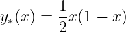
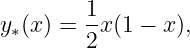
Then
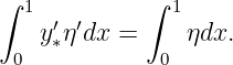
Integrating the first term by parts,
The boundary term vanishes because η(0) = η(1) = 0, and y∗′′ = −1, so
Therefore
for every admissible variation.
Solution 3: weighted arc-length functionalThe integrand is
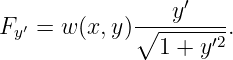
Differentiate with respect to y:
Differentiate with respect to y′:
Hence
When w = 1, the displacement term disappears and
This is the first-variation starting point for the shortest-path problem.
Solution 4: mechanical actionThe mechanical integrand is the Lagrangian
Under
the first variation is
For the harmonic oscillator,
so
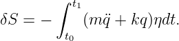
Integrate the first term by parts:
Because the endpoint variations vanish,
Any trajectory satisfying
therefore gives
for every admissible η.
Figure. Hamilton’s principle uses exactly the same first-variation machinery as the abstract functional problem: perturb the trajectory while fixing the endpoint events, then differentiate the action with respect to the perturbation amplitude.
Solution 5: two coupled dependent variablesPerturb both variables:
Then
Differentiating the scalarized functional at 𝜖 = 0 gives
The two variations are independent. Later, the vector version of the Euler–Lagrange equation will turn the coefficients of η and ξ into a coupled system of differential equations.
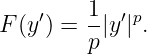
Solution 6: the p-energyLet
For p > 1, the derivative with respect to y′ is
There is no explicit dependence on y, so Fy = 0. Therefore
For p = 2,
For p = 4,
If instead one omits the prefactor 1∕p and uses J = ∫ y′4dx, the corresponding first variation is 4 ∫ y′3η′dx, matching the direct expansion in CV02E1.
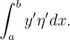
Solution 7: adding a total derivativeWrite
Under a variation, the first term contributes
The boundary contribution varies as
For fixed endpoints,
so this term vanishes. Hence
Thus a total derivative changes only endpoint data. When endpoint values are fixed, it does not alter the interior stationarity equation. In mechanics, this is the familiar fact that Lagrangians differing by a total time derivative produce the same equations of motion.
Figure. Adding a total derivative changes the action by a boundary contribution. For fixed endpoints its first variation vanishes, leaving the interior variational condition unchanged.
Solution 8: explicit x dependenceThe integrand is
Therefore
The first variation is
For y = 0, both y and y′ vanish identically, so
for every admissible variation. Thus y = 0 is stationary. Because the integrand is nonnegative and vanishes at y = 0, one can in this special case go further and identify it as a global minimizer, but that conclusion uses more than the first variation alone.
3 SummaryFor the classical first-order functional
the practical workflow is
The examples show that the same structure covers elastic-energy-like functionals, forced boundary-value problems, path length, mechanical action, coupled coordinates, nonlinear p-energies, and Lagrangians modified by total derivatives. The first variation is therefore the common language connecting a large class of physical extremum principles. "Calculus of Variations: First Variations of Common Functionals" is owned by bloftin.
This object's parent. Cross-references: system of differential equations, vector, amplitude, Hamilton's principle, Lagrangian, boundary, displacement, energy, oscillator, harmonic, particle, function, mechanics, formula, CV02E1 This is version 1 of Calculus of Variations: First Variations of Common Functionals, born on 2026-09-10. Object id is 1144, canonical name is CalculusOfVariationsFirstVariationsOfCommonFunctionals. Accessed 272 times total. Classification:
|
|
|
|
Pending Errata and AddendaNone.
|
DiscussionNo messages.
|
Interact |
![[parent]](https://images.physicslibrary.org/images/uparrow.png)
![∫ b
δJ [y;η ] = (F η + F ′η′) dx
a y y](https://images.physicslibrary.org/cache/objects/1144/make4ht/CalculusOfVariationsFirstVariationsOfCommonFunctionals0x.png)

![∫ [ ]
b 1- ′2
J[y] = 2 a(x)y + V (x,y) dx,
a](https://images.physicslibrary.org/cache/objects/1144/make4ht/CalculusOfVariationsFirstVariationsOfCommonFunctionals1x.png)
![∫ 1[1 ]
J[y] = --y′2 − f(x )y dx
0 2](https://images.physicslibrary.org/cache/objects/1144/make4ht/CalculusOfVariationsFirstVariationsOfCommonFunctionals2x.png)
![∫ b ∘ -------
J[y] = w (x,y) 1 + y′2dx,
a](https://images.physicslibrary.org/cache/objects/1144/make4ht/CalculusOfVariationsFirstVariationsOfCommonFunctionals4x.png)
![∫ t1[ ]
S[q] = 1-m ˙q2 − V(q,t) dt.
t0 2](https://images.physicslibrary.org/cache/objects/1144/make4ht/CalculusOfVariationsFirstVariationsOfCommonFunctionals5x.png)


![∫ b[ 1 1 ]
J[u,v] = -u′2 + -v′2 + cuv dx.
a 2 2](https://images.physicslibrary.org/cache/objects/1144/make4ht/CalculusOfVariationsFirstVariationsOfCommonFunctionals8x.png)
![∫
1 b ′ p
Jp[y ] =-- |y | dx.
p a](https://images.physicslibrary.org/cache/objects/1144/make4ht/CalculusOfVariationsFirstVariationsOfCommonFunctionals9x.png)
![δJp [y;η ].](https://images.physicslibrary.org/cache/objects/1144/make4ht/CalculusOfVariationsFirstVariationsOfCommonFunctionals10x.png)
![∫ [ ]
^ b 1-′2 d--
J [y] = 2y + dxG (x,y ) dx,
a](https://images.physicslibrary.org/cache/objects/1144/make4ht/CalculusOfVariationsFirstVariationsOfCommonFunctionals11x.png)
![∫ b
δJ^[y;η] = y′η′dx.
a](https://images.physicslibrary.org/cache/objects/1144/make4ht/CalculusOfVariationsFirstVariationsOfCommonFunctionals12x.png)
![∫ [ ]
2 1- 2 ′2 1-x 2
J [y] = 2x y + 2e y dx.
1](https://images.physicslibrary.org/cache/objects/1144/make4ht/CalculusOfVariationsFirstVariationsOfCommonFunctionals13x.png)


![|--------------------------------------|
| ∫ b |
|δJ[y;η] = [Vy(x, y)η + a(x)y′η ′]dx. |
------------a--------------------------](https://images.physicslibrary.org/cache/objects/1144/make4ht/CalculusOfVariationsFirstVariationsOfCommonFunctionals16x.png)


![|------------------------------|
| ∫ 1 |
|δJ[y;η] = [y′η′ − f(x )η ]dx.
------------0-------------------](https://images.physicslibrary.org/cache/objects/1144/make4ht/CalculusOfVariationsFirstVariationsOfCommonFunctionals19x.png)

![∫ 1[ ( 1 ) ]
δJ[y∗;η] = -− x η′ − η dx.
0 2](https://images.physicslibrary.org/cache/objects/1144/make4ht/CalculusOfVariationsFirstVariationsOfCommonFunctionals22x.png)
![∫ ∫
1 ′ ′ ′ 1 1 ′′
y∗ηdx = [y∗η]0 − y∗ηdx.
0 0](https://images.physicslibrary.org/cache/objects/1144/make4ht/CalculusOfVariationsFirstVariationsOfCommonFunctionals23x.png)
![|------------|
-δJ[y∗;η] =-0-](https://images.physicslibrary.org/cache/objects/1144/make4ht/CalculusOfVariationsFirstVariationsOfCommonFunctionals25x.png)


![|----------∫-b[-----------------------------]----|
| ∘ ------′2 ----y′--- ′ |
|δJ[y;η] = a wy 1 + y η + w ∘ 1 + y′2η dx. |
--------------------------------------------------](https://images.physicslibrary.org/cache/objects/1144/make4ht/CalculusOfVariationsFirstVariationsOfCommonFunctionals29x.png)
![|----------------------------|
| ∫ b y′ |
|δJ[y;η] = ∘--------η′dx. |
------------a----1-+-y′2------|](https://images.physicslibrary.org/cache/objects/1144/make4ht/CalculusOfVariationsFirstVariationsOfCommonFunctionals30x.png)


![|----------------------------------|
| ∫ t1 |
|δS[q;η] = [m ˙q ˙η − Vq(q,t)η]dt.
------------t0----------------------](https://images.physicslibrary.org/cache/objects/1144/make4ht/CalculusOfVariationsFirstVariationsOfCommonFunctionals33x.png)

![∫
t1
δS = [m ˙q˙η − kqη]dt.
t0](https://images.physicslibrary.org/cache/objects/1144/make4ht/CalculusOfVariationsFirstVariationsOfCommonFunctionals35x.png)
![∫ ∫
t1 t1 t1
m ˙q˙ηdt = [m ˙qη]t0 − m ¨qηdt.
t0 t0](https://images.physicslibrary.org/cache/objects/1144/make4ht/CalculusOfVariationsFirstVariationsOfCommonFunctionals36x.png)





![|---------------∫------------------------------|
| b ′ ′ ′ ′ |
|δJ [u,v; η,ξ] = [uη + v ξ + c(vη + uξ)]dx. |
-----------------a-----------------------------](https://images.physicslibrary.org/cache/objects/1144/make4ht/CalculusOfVariationsFirstVariationsOfCommonFunctionals42x.png)

![|----------∫-b--------------|
| ′ p− 2 ′′ |
δJp[y;η] = a |y | y η dx. |
-----------------------------](https://images.physicslibrary.org/cache/objects/1144/make4ht/CalculusOfVariationsFirstVariationsOfCommonFunctionals45x.png)
![∫
b ′′
δJ2[y;η] = yη dx.
a](https://images.physicslibrary.org/cache/objects/1144/make4ht/CalculusOfVariationsFirstVariationsOfCommonFunctionals46x.png)
![∫ b
δJ4[y;η] = y′3η′dx.
a](https://images.physicslibrary.org/cache/objects/1144/make4ht/CalculusOfVariationsFirstVariationsOfCommonFunctionals47x.png)
![∫ b1
^J[y] = -y ′2dx + G (b,y(b)) − G (a,y(a)).
a 2](https://images.physicslibrary.org/cache/objects/1144/make4ht/CalculusOfVariationsFirstVariationsOfCommonFunctionals48x.png)
![δ[G(b,y(b)) − G (a, y(a))] = Gy (b,y(b))η (b) − Gy (a,y(a))η(a).](https://images.physicslibrary.org/cache/objects/1144/make4ht/CalculusOfVariationsFirstVariationsOfCommonFunctionals50x.png)

![|--------------------|
| ∫ b |
|δ ^J[y;η] = y′η′dx.|
------------a---------](https://images.physicslibrary.org/cache/objects/1144/make4ht/CalculusOfVariationsFirstVariationsOfCommonFunctionals52x.png)



![|--------------------------------|
| ∫ 2[ ] |
|δJ[y;η] = exy η + x2y′η ′dx. |
------------1---------------------](https://images.physicslibrary.org/cache/objects/1144/make4ht/CalculusOfVariationsFirstVariationsOfCommonFunctionals55x.png)
![|------------|
|δJ [0;η] = 0 |
-------------](https://images.physicslibrary.org/cache/objects/1144/make4ht/CalculusOfVariationsFirstVariationsOfCommonFunctionals56x.png)
![∫ b
J [y] = F (x,y,y ′)dx,
a](https://images.physicslibrary.org/cache/objects/1144/make4ht/CalculusOfVariationsFirstVariationsOfCommonFunctionals57x.png)
![∫ b
F −→ (Fy,Fy ′) −→ δJ [y;η] = (Fyη + Fy ′η ′)dx.
a](https://images.physicslibrary.org/cache/objects/1144/make4ht/CalculusOfVariationsFirstVariationsOfCommonFunctionals58x.png)