Calculus of Variations: Euler–Lagrange Introductory Exercises and Worked Solutions
This companion entry turns the Euler–Lagrange equation from CV04 into a repeatable
problem-solving procedure. The goal is not to memorize
but to become comfortable reading a functional, computing the two partial derivatives, taking the
required total derivative with respect to the independent variable, imposing endpoint data, and
interpreting what the result actually proves.
The exercises begin with direct substitutions and linear boundary-value problems. They then
introduce a nonlinear integrand, reverse-engineering a Lagrangian from a differential equation,
and a final example showing that a stationary function can be a saddle rather than a
minimum.
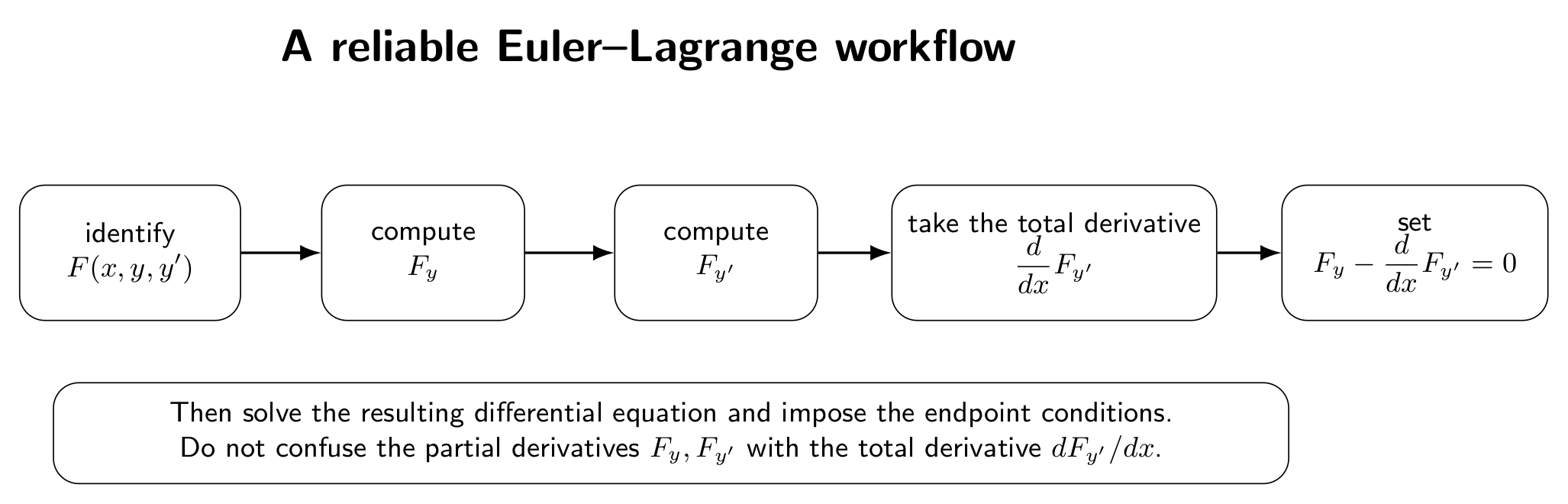
Figure. A reliable Euler–Lagrange workflow. The derivative in the fourth box is a total
derivative along the candidate curve; this is the step most likely to be compressed too
aggressively in a first calculation.
1 Exercises
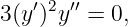
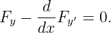
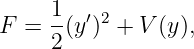
Exercise 1: identify the Euler–Lagrange ingredients
For each integrand below, compute Fy, Fy′, and dFy′∕dx, then write the Euler–Lagrange
differential equation. Do not solve the resulting equation unless it is immediate.
-
-
-
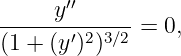
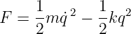
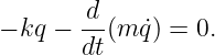
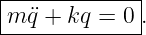
- With the independent variable interpreted as time t,
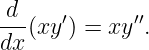
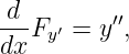
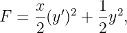
For part (b), explicitly identify the product-rule term that would be missed if one incorrectly
wrote
Exercise 2: Dirichlet energy and the straight-line extremal
Consider
on the fixed-endpoint class
- Derive the Euler–Lagrange equation.
- Solve the resulting boundary-value problem.
- Evaluate J on the stationary curve.
- Go beyond Euler–Lagrange and prove directly that this stationary curve is the
global minimizer by writing an arbitrary admissible function as y = x + u, where
u(0) = u(1) = 0.
Explain carefully which part of the argument establishes stationarity and which part establishes
the stronger statement of global minimum.
Exercise 3: a static quadratic energy with a restoring term
Let
with
- Derive the Euler–Lagrange equation.
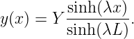
- Define λ =
 and solve the boundary-value problem.
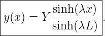
- Show that the solution can be written
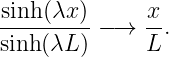
- Examine the limit K → 0 and show that the solution approaches a straight line.
Exercise 4: uniformly forced string or membrane strip
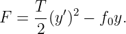
Consider
with fixed endpoints
- Derive the Euler–Lagrange equation.
- Solve for y(x).
- Locate the maximum displacement and find its value.
- Explain why the sign of the curvature is consistent with the sign convention used in
the potential term −f0y.
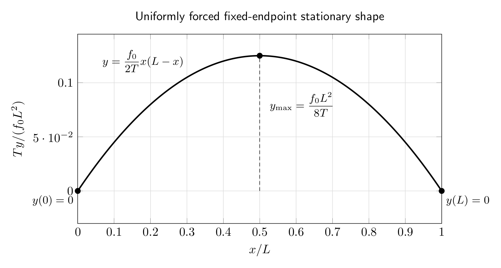
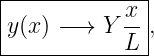
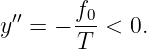
Figure. For a constant load f0 > 0, the Euler–Lagrange equation gives a parabolic
stationary shape. The fixed endpoints determine the two integration constants after the
differential equation has been obtained.
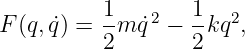
Exercise 5: harmonic oscillator from stationary action
Let
with
- Derive the Euler–Lagrange equation.
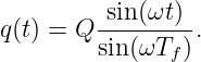
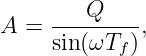
- Define ω =
 and solve the equation.
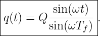
- Assuming sin(ωTf)≠0, show that the unique stationary path satisfying the endpoints
is
- What special feature occurs when sin(ωTf) = 0? Explain why this is a boundary-value issue
rather than a failure of the Euler–Lagrange equation.
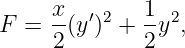
Exercise 6: explicit x-dependence and the total derivative
Consider
- Compute Fy and Fy′.
- Expand dFy′∕dx one algebraic step at a time.
- Show that the Euler–Lagrange equation is
- Explain why replacing dFy′∕dx by the partial derivative ∂Fy′∕∂x would also give the wrong
result in a general problem where Fy′ depends on y or y′.
Exercise 7: a nonlinear derivative energy
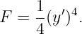
Let
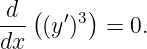
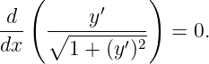
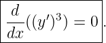
- Derive the Euler–Lagrange equation in the form
- Integrate this equation before expanding it and determine the stationary curve.
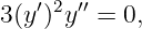
- If one expands the equation as
why is dividing immediately by (y′)2 a logically unnecessary and potentially misleading
step?
- Evaluate J on the stationary curve.
Exercise 8: reverse-engineer a Lagrangian
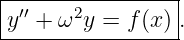
Suppose one wants the Euler–Lagrange equation to reproduce the forced linear oscillator
equation
- Show that
produces the desired equation.
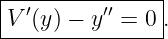
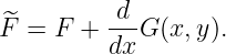
- Explain why adding a constant to F does not change the Euler–Lagrange equation.
- Verify directly that adding the total derivative dG(x,y)∕dx to F changes the action only by
endpoint terms when the endpoints are fixed.
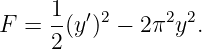
Exercise 9: stationary does not mean minimum
Consider
- Show that y∗ = 0 satisfies the Euler–Lagrange equation and is therefore stationary.
- Evaluate J on the one-parameter family
- Evaluate J on the one-parameter family
- Use the two signs obtained above to classify y∗ = 0 locally along these two directions. Why
does the Euler–Lagrange equation alone not contain this classification information?
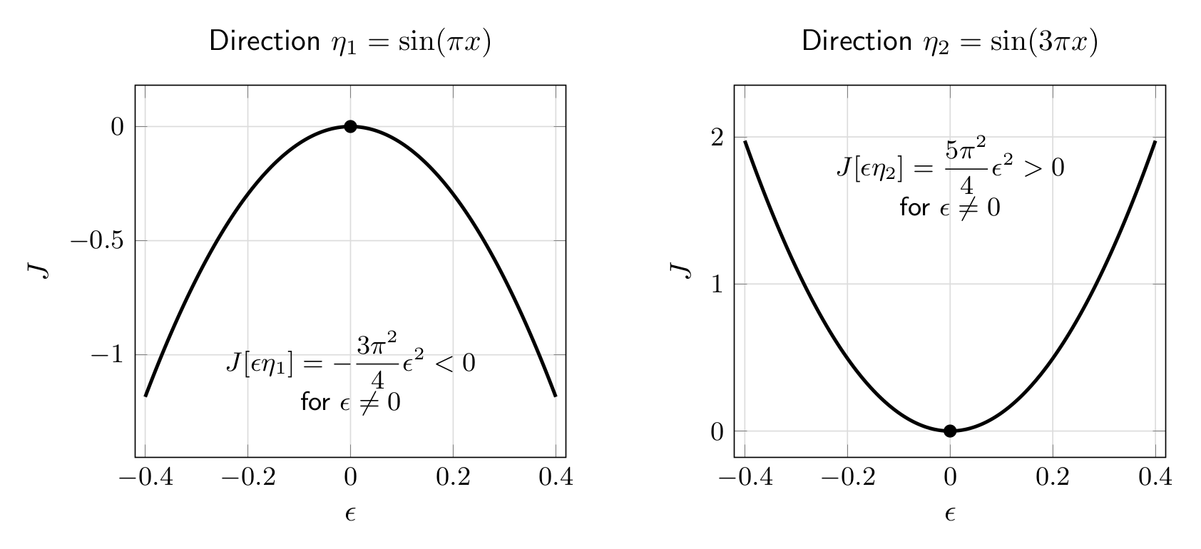
Figure. The same stationary function y∗ = 0 can be approached along directions that
decrease J and directions that increase J. The Euler–Lagrange equation detects
stationarity, not this second-order classification.
2 Solutions
Solution 1: identify the Euler–Lagrange ingredients
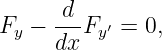
The Euler–Lagrange equation is
(a) For
we have
Hence
and the Euler–Lagrange equation is
(b) For
we obtain
Now the product rule is essential:
Therefore
or
The term y′ is exactly the term lost by the incorrect replacement d(xy′)∕dx = xy′′.
(c) For
we have
Thus
Differentiating gives
so any regular stationary graph satisfies
(d) Treating t as the independent variable,
gives
Hence
For constant m,
Solution 2: Dirichlet energy and the straight-line extremal
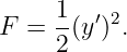
The integrand is
Therefore
Euler–Lagrange gives
so
Integrating twice,
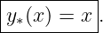
The endpoint y(0) = 0 gives C2 = 0, and y(1) = 1 gives C1 = 1. Thus
Its functional value is
The Euler–Lagrange calculation has established stationarity. To prove the global minimum, let any
admissible competitor be written
Then
| J[y] | =  ∫
01(1 + u′)2 dx ∫
01(1 + u′)2 dx | (54)
|
| =  + ∫
01u′dx + + ∫
01u′dx +  ∫
01(u′)2 dx. ∫
01(u′)2 dx. | (55) |
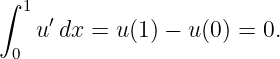
The middle term vanishes because
Hence
Therefore
The distinction is important: Euler–Lagrange found the candidate; positivity of the remainder
proved the minimum.
Solution 3: a static quadratic energy with a restoring term
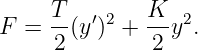
Here
Thus
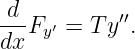
With constant T,
Therefore
or
The general solution is
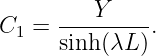
The condition y(0) = 0 gives C2 = 0. Then
so
Hence
As K → 0, λ → 0. Using sinh z ∼ z,
Thus
which is the straight-line extremal recovered when the restoring term is removed.
Solution 4: uniformly forced string or membrane strip
The integrand is
Therefore
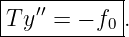
Euler–Lagrange gives
so
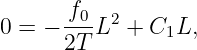
Integrating twice,
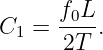
From y(0) = 0, C2 = 0. From y(L) = 0,
so
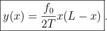
Thus
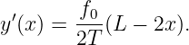
Differentiate:
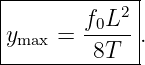
The maximum occurs at
and
Because f0 > 0 appears in the functional as −f0y, increasing y lowers that potential contribution.
The stationary curve therefore bows in the positive y direction, while its second derivative is
negative:
Solution 5: harmonic oscillator from stationary action
With
we have
The Euler–Lagrange equation is
or
The general solution is
The condition q(0) = 0 gives B = 0. The final condition gives
If sin(ωTf)≠0, then
and therefore
If sin(ωTf) = 0, the endpoint condition becomes
Thus, for Q≠0, no solution of the Euler–Lagrange ODE can satisfy those two endpoints. For Q = 0,
infinitely many amplitudes A satisfy the endpoint conditions. This is a special property of the
boundary-value problem at those time intervals, not a breakdown of Euler–Lagrange
theory.
Solution 6: explicit x-dependence and the total derivative
For
we have
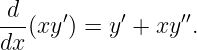
Now expand the total derivative carefully:
 Fy′ Fy′ | =  (xy′) (xy′) | (93)
|
| =  y′ + x y′ + x | (94)
|
| = y′ + xy′′. | (95) |
Therefore
which is
The distinction between partial and total derivatives matters because, in general,
Consequently,
The partial derivative ∂Fy′∕∂x holds y and y′ fixed; the total derivative follows their variation
along the candidate curve.
Solution 7: a nonlinear derivative energy
Here
Thus
Euler–Lagrange gives
Integrate before expanding:
Since the real cube root is single valued,
so
The endpoints give B = 0 and A = 1, hence
If instead we first expand,
then dividing by (y′)2 assumes y′≠0. That assumption has not yet been established
and is unnecessary. The integrated equation (y′)3 = C is cleaner and loses no possible
branch.
Finally,
Solution 8: reverse-engineer a Lagrangian
Take
Then
Euler–Lagrange gives
or
Adding a constant C to F changes neither Fy nor Fy′, so the Euler–Lagrange equation is
unchanged.
More generally, let
The corresponding functional changes by
| J[y] − J[y] | = ∫
ab G(x,y(x)) dx G(x,y(x)) dx | (114)
|
| = G(b,y(b)) − G(a,y(a)). | (115) |
For fixed endpoint values this difference is the same for every admissible curve, so the interior
stationarity equation is unchanged.
Solution 9: stationary does not mean minimum
The integrand is
Therefore
The Euler–Lagrange equation is
or
Clearly y∗ = 0 satisfies this equation and the endpoint conditions, so it is stationary.
Now take
Then
Using
we obtain
| J[𝜖 sin(πx)] | =  ![[ ]
2 2 1 2 21
𝜖 π 2 − 4π 𝜖 2-](https://images.physicslibrary.org/cache/objects/1199/make4ht/CalculusOfVariationsEulerLagrangeIntroductoryExercisesAndWorkedSolutions126x.png) | (123)
|
| = − 𝜖2 . 𝜖2 . | (124) |
Thus this direction decreases J below J[0] = 0.
For
we have
so
| J[𝜖 sin(3πx)] | =  ![[ 1 1 ]
9π2 𝜖2 -− 4π2𝜖2--
2 2](https://images.physicslibrary.org/cache/objects/1199/make4ht/CalculusOfVariationsEulerLagrangeIntroductoryExercisesAndWorkedSolutions131x.png) | (127)
|
| =  𝜖2 . 𝜖2 . | (128) |
This direction increases J above zero. Hence arbitrarily close to y∗ = 0 there are admissible
functions with both larger and smaller functional values. The stationary function is therefore
saddle-like rather than a local minimum or maximum.
The Euler–Lagrange equation is a first-order stationarity condition in function space. Classification
requires additional information, such as the second variation developed later in the
series.
3 Summary
The exercises establish a reusable Euler–Lagrange workflow:
The most important conceptual points are equally reusable:
- the derivative dFy′∕dx is a total derivative along the candidate curve;
- endpoint conditions are imposed after the Euler–Lagrange differential equation has
been obtained in the fixed-endpoint problem;
- nonlinear Euler–Lagrange equations are often safer to integrate in an unexpanded form
before dividing by quantities that might vanish; and
- satisfying Euler–Lagrange proves stationarity, not minimum classification.
CV04E2 can now specialize these tools to shortest-path problems, while CV04E3 can emphasize
nonlinear integrands and more demanding algebra.
Further reading
For complementary treatments of the Euler–Lagrange equation and classical variational problems,
see I. M. Gelfand and S. V. Fomin, Calculus of Variations; Robert Weinstock, Calculus of
Variations with Applications to Physics and Engineering; Hans Sagan, Introduction
to the Calculus of Variations; and Cornelius Lanczos, The Variational Principles of
mechanics. These references are useful for comparing notation and for seeing how the same
Euler–Lagrange structure appears in analysis, mechanics, geometry, and mathematical
physics.

![[parent]](https://images.physicslibrary.org/images/uparrow.png)




![∫ 1
J [y] = 1- y′(x)2 dx
2 0](https://images.physicslibrary.org/cache/objects/1199/make4ht/CalculusOfVariationsEulerLagrangeIntroductoryExercisesAndWorkedSolutions6x.png)
![𝒜 = {y ∈ C2 ([0,1]) : y(0) = 0, y(1) = 1} .](https://images.physicslibrary.org/cache/objects/1199/make4ht/CalculusOfVariationsEulerLagrangeIntroductoryExercisesAndWorkedSolutions7x.png)
![∫ L [T K ]
J [y] = --(y′)2 +---y2 dx, T > 0, K > 0,
0 2 2](https://images.physicslibrary.org/cache/objects/1199/make4ht/CalculusOfVariationsEulerLagrangeIntroductoryExercisesAndWorkedSolutions8x.png)

![∫ L[ T ]
J [y] = --(y ′)2 − f0y dx, T > 0,
0 2](https://images.physicslibrary.org/cache/objects/1199/make4ht/CalculusOfVariationsEulerLagrangeIntroductoryExercisesAndWorkedSolutions12x.png)

![∫ [ ]
Tf 1 2 1 2
S[q] = --m ˙q − -kq dt,
0 2 2](https://images.physicslibrary.org/cache/objects/1199/make4ht/CalculusOfVariationsEulerLagrangeIntroductoryExercisesAndWorkedSolutions14x.png)

![∫ 2 [x 1 ]
J [y] = --(y ′)2 + -y2 dx.
1 2 2](https://images.physicslibrary.org/cache/objects/1199/make4ht/CalculusOfVariationsEulerLagrangeIntroductoryExercisesAndWorkedSolutions18x.png)

![∫
1- 1 ′ 4
J [y ] = 4 y(x ) dx, y(0) = 0, y(1) = 1.
0](https://images.physicslibrary.org/cache/objects/1199/make4ht/CalculusOfVariationsEulerLagrangeIntroductoryExercisesAndWorkedSolutions20x.png)


![∫
1 1[ ′ 2 2 2]
J [y] = -- (y ) − 4π y dx, y(0) = y (1 ) = 0.
2 0](https://images.physicslibrary.org/cache/objects/1199/make4ht/CalculusOfVariationsEulerLagrangeIntroductoryExercisesAndWorkedSolutions25x.png)














![∫ |--|
1 1 |1 |
J[y∗] = -- 1 dx = |--.
2 0 -2-](https://images.physicslibrary.org/cache/objects/1199/make4ht/CalculusOfVariationsEulerLagrangeIntroductoryExercisesAndWorkedSolutions53x.png)

![∫ 1
J [y] = 1-+ 1- (u ′)2dx ≥ 1.
2 2 0 2](https://images.physicslibrary.org/cache/objects/1199/make4ht/CalculusOfVariationsEulerLagrangeIntroductoryExercisesAndWorkedSolutions59x.png)


























![∫ 1 |--|
J[y ] = 1- 1 dx = |1-.
∗ 4 0 -4-|](https://images.physicslibrary.org/cache/objects/1199/make4ht/CalculusOfVariationsEulerLagrangeIntroductoryExercisesAndWorkedSolutions111x.png)











![∫ b
J [y] = F(x,y, y′) dx =⇒ Fy, Fy′, -d-Fy′, Fy − d-Fy ′ = 0.
a dx dx](https://images.physicslibrary.org/cache/objects/1199/make4ht/CalculusOfVariationsEulerLagrangeIntroductoryExercisesAndWorkedSolutions133x.png)