Wave Scattering, Inhomogeneities, and the Born Approximation
The earlier wave articles treated propagation in uniform media, reflection at sharp interfaces,
normal modes in bounded regions, and forced response.
A new effect appears when the medium varies through space.
A wave entering an inhomogeneous region can generate a new outgoing field.
That process is wave scattering.
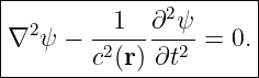
We begin with a scalar wave equation whose local wave speed depends on position:
For harmonic time dependence,
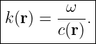
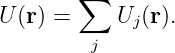
the spatial field satisfies
where
Choose a uniform background medium with wave speed
and wave number
Define the scattering potential
Then
The inhomogeneity therefore acts like a distributed source whose strength depends on the field
itself.
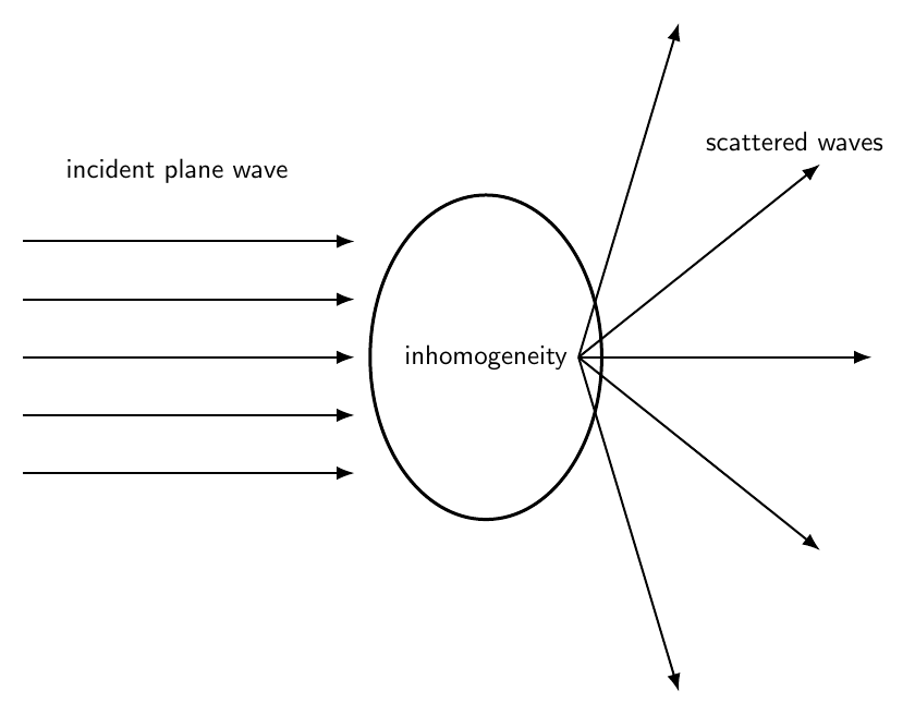
Figure 1. An incident plane wave enters a localized inhomogeneity. The total field is written as an
incident field plus an outgoing scattered field.
1 Incident, scattered, and total fields
Write
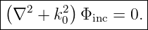
The incident field is a solution of the background equation:
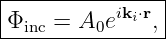
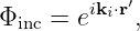
For a plane incident wave,
with
The scattered field is the additional field produced by the inhomogeneity.
For an isolated scatterer in open space, the physical scattered solution must be outgoing.
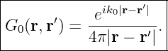
2 Outgoing free-space Green function
The background Helmholtz Green function is defined by
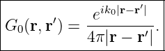
In three dimensions, the outgoing solution is
The outgoing exponential selects waves propagating away from the source point
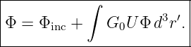
3 The Lippmann-Schwinger equation
Starting from
use the Green function to write
This is the Lippmann-Schwinger equation for the scalar scattering problem.
It has an important physical interpretation.
The total field inside the inhomogeneity drives secondary outgoing waves.
Those secondary waves add to the incident field to produce the total field.
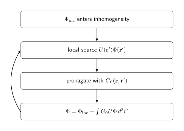
Figure 3. The Lippmann-Schwinger equation is an integral equation because the field inside the
scatterer both responds to the incident wave and becomes the source of the scattered wave.
4 Why the scattering problem is implicit
The integral contains
the unknown total field.
Therefore the equation does not merely evaluate the scattered wave from a known source.
The source itself depends on the unknown field.
Strong scattering can therefore include repeated interactions:
- the incident field excites the inhomogeneity,
- the generated field propagates,
- that field interacts with the inhomogeneity again,
- further scattered contributions are produced.
This repeated interaction is multiple scattering.
5 Born series
Insert the Lippmann-Schwinger equation back into itself.
Symbolically,
One iteration gives
Continuing formally,
| Φ | = Φinc + G0UΦinc | (21)
|
| + G0UG0UΦinc +  . | (22) |
This is the Born series.
The terms represent:
- zeroth order: incident wave,
- first order: one scattering interaction,
- second order: two scattering interactions,
- higher orders: repeated scattering.
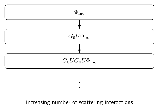
Figure 4. The Born series organizes the total field by number of scattering interactions. The first
Born approximation retains only the incident wave inside the scattering integral.
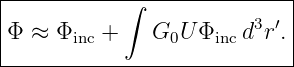
6 First Born approximation
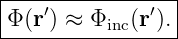
If the inhomogeneity is sufficiently weak, the field inside the scattering region remains close to the
incident field:
Then
This is the first Born approximation.
It is a single-scattering approximation.
It neglects the modification of the internal field by repeated scattering.
7 Far-field approximation
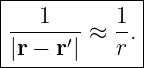
Suppose the scatterer is localized near the origin and the observation point is far away:
Then
and
Therefore
| G0(r,r′) | ≈ e−ik0r⋅r′. | (28) |
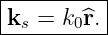
Define the scattered wave vector
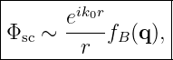
8 Scattering amplitude
For an incident plane wave of unit amplitude,
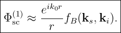
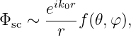
the far-field Born scattered wave becomes
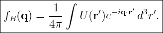
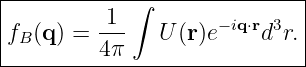
The first Born scattering amplitude is
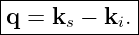
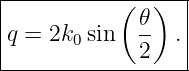
Define the momentum-transfer or scattering vector
Then
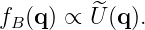
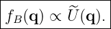
The Born scattering amplitude is therefore the spatial Fourier transform of the scattering
potential, apart from the factor
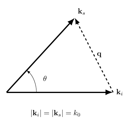
Figure 2. Elastic scalar scattering conserves wave-number magnitude in the uniform background.
The vector q = ks − ki measures the spatial frequency sampled by the scattering process.
9 Magnitude of the scattering vector
For elastic scattering,
If
is the angle between
and
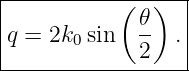
then
| q2 | = |k
s − ki|2 | (40)
|
| = k02 + k
02 − 2k
02 cos 𝜃 | (41)
|
| = 2k02(1 − cos 𝜃). | (42) |
Using
we obtain
Forward scattering has
Backscattering has
10 Scattering as spatial-frequency measurement
The first Born amplitude has the form
Therefore changing the scattering angle changes the spatial Fourier component of the
inhomogeneity that is sampled.
Small angles correspond to small
and therefore large-scale structure.
Large angles correspond to larger
and therefore finer spatial structure.
This Fourier-transform interpretation is fundamental in diffraction, imaging, radar, acoustics, and
many inverse problems.
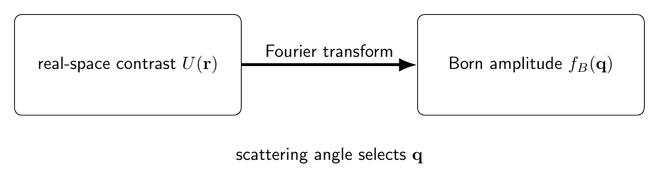
Figure 5. In the first Born approximation, each scattering direction samples one Fourier
component of the inhomogeneity. Changing angle changes the scattering vector q.
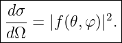
11 Differential scattering cross section
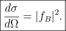
If the incident plane wave has unit amplitude and the scattered far field is
the differential scattering cross section is
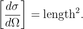
The dimensions are:
and
Since
the Born integral indeed gives
12 Spherically symmetric scatterer
Suppose
Choose the
axis along
Then
The angular integral gives
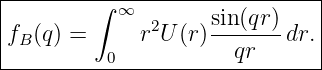
Therefore
The three-dimensional Fourier transform has reduced to a one-dimensional radial integral.
13 Example 1: Gaussian inhomogeneity
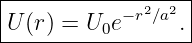
Consider
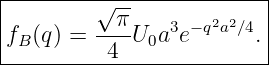
The three-dimensional Fourier transform is
Therefore
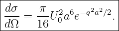
The differential cross section is
The scattering becomes increasingly forward-peaked when
is large because larger scattering angles correspond to larger
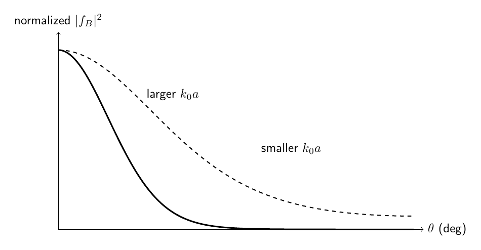
Figure 6. A smooth Gaussian inhomogeneity has a smooth Gaussian Fourier transform. Increasing
the size parameter k0a narrows the angular scattering pattern toward the forward direction.
14 Example 2: uniform spherical inhomogeneity
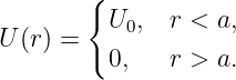
Let
Then
| fB(q) | = U0 ∫
0ar2 dr. | (69) |
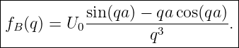
Evaluating the integral gives
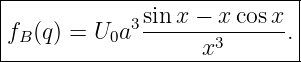
Equivalently, with
15 Forward limit of the uniform sphere
As
use
and
Then
Therefore
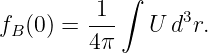
This also follows directly from
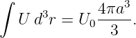
For a uniform sphere,
16 Example 3: numerical sphere amplitude
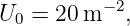
Take
and
At
| q | = 2k0 sin 30∘ | (84)
|
| = 10.0 m−1. | (85) |
Therefore
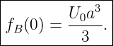
The Born amplitude is
| fB | = U0a3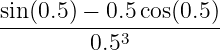 | (87)
|
| ≈ 8.13 × 10⁻⁴ m. | (88) |
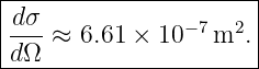
The differential cross section is approximately
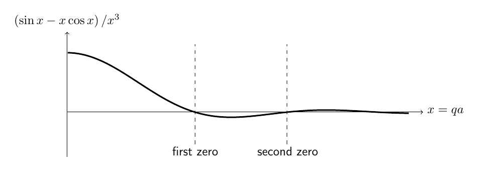
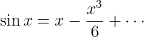
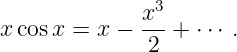
Figure 7. The uniform sphere has an oscillatory form factor. Destructive interference produces
angular minima when sinx − xcosx = 0, with x = qa.
17 Why scattering minima appear
Different parts of an extended scatterer radiate secondary waves with different phases.
At some observation angles, these contributions reinforce.
At others, they cancel.
The oscillatory factor
is therefore an interference effect across the finite sphere.
Scattering patterns contain information about scatterer size and shape because of this internal
phase structure.
18 Born validity
The first Born approximation assumes
inside the scattering region.
It is best when:
- the contrast is weak,
- the scatterer is not too large in accumulated phase shift,
- multiple scattering is small,
- the system is not near a strong internal Resonance.
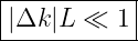
A useful heuristic is that the phase perturbation through the object should remain
small.
If
is a characteristic change in wave number and
is a characteristic traversal length, one often wants
for a comfortably weak phase perturbation.
This is a heuristic, not a universal theorem.
Different scattering geometries can require more careful validity criteria.
19 A dimensionless weak-scattering estimate
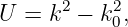
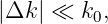
Since
if
with
then
| U | = (k0 + Δk)2 − k
02 | (98)
|
| ≈ 2k0Δk. | (99) |
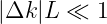
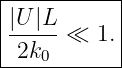
Therefore a rough small-phase condition
can also be written approximately as
Again, this is an order-of-magnitude guide.
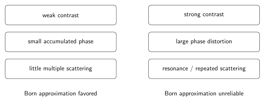
Figure 8. The first Born approximation is most reliable when the internal field remains close to
the incident field. Strong contrast, long accumulated phase, repeated scattering, or internal
resonance can invalidate the approximation.
20 When the first Born approximation fails
Important failure mechanisms include:
- strong wave-speed contrast,
- large accumulated phase through the scatterer,
- repeated internal reflection,
- multiple scattering among separated objects,
- resonant trapping or cavity-like behavior,
- very strong forward phase distortion.
Then higher Born terms or a different solution method may be required.
Possible approaches include:
- retaining additional Born-series terms,
- direct numerical solution of the Helmholtz equation,
- boundary-element methods,
- finite-element methods,
- exact partial-wave methods for symmetric scatterers.
21 Relation to sharp-interface reflection
The earlier interface articles treated an abrupt material boundary.
Scattering from a distributed inhomogeneity generalizes that idea.
A sharp interface can be viewed as an extreme spatial variation.
A weak smooth inhomogeneity instead produces many small secondary contributions distributed
throughout its volume.
The Born approximation sums those weak contributions coherently.
22 Relation to diffraction
Diffraction and scattering are closely related wave phenomena.
Both involve:
In the first Born approximation, the connection becomes explicit:
This is the same mathematical structure that appears in far-field diffraction from apertures and
objects.
23 Relation to quantum scattering
The time-independent Schrödinger equation can also be rearranged into a Helmholtz-like equation
containing a potential term.
That produces a mathematically similar Lippmann-Schwinger equation and Born approximation.
The interpretation is different:
- here Φ is a classical scalar wave amplitude,
- in quantum mechanics the wavefunction has a probabilistic interpretation.
The mathematical analogy is nevertheless extremely useful.
24 Scattering from several weak objects
Suppose
In the first Born approximation,
| fB(q) | =  ∫
∑
jUj(r)e−iq⋅rd3r | (104)
|
| = ∑
jfB,j(q). | (105) |
Thus the amplitudes add before taking the squared magnitude.
The resulting cross section contains interference terms between different scatterers.
This is why arrays, lattices, and distributed targets can produce sharp angular structure.
25 Translated identical scatterers
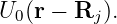
Let one scatterer have potential
If a copy is translated to
its potential is
Its Fourier transform gains a phase:
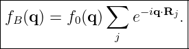
For many identical scatterers,
The first factor describes one object.
The second factor describes the arrangement of objects.
This is the basic separation between a form factor and a structure factor.
26 Common mistakes
- Forgetting that the total field is incident plus scattered field.
- Defining the scattering potential with one sign and then using formulas derived for the
opposite sign.
- Forgetting the outgoing boundary condition on the Green function.
- Treating the Lippmann-Schwinger equation as explicit even though the unknown field
appears inside the integral.
- Calling the first Born approximation an exact solution.
- Replacing the internal field by zero rather than by the incident field.
- Forgetting the far-field approximation when defining a scattering amplitude.
- Using q = ki − ks while keeping an exponential convention derived for q = ks − ki.
- Forgetting that q = 2k0 sin(𝜃∕2) for elastic scattering.
- Confusing amplitude with differential cross section.
- Forgetting that dσ∕dΩ = |f|2 has units of area.
- Treating large-angle scattering as sampling only large spatial scales.
- Forgetting the factor sin(qr)∕(qr) for a spherical Fourier transform.
- Using the sphere formula directly at q = 0 without taking its finite limit.
- Applying the Born approximation to strong or resonant scatterers without checking
validity.
27 Practice exercises
- Starting from a spatially varying wave speed, derive the Helmholtz scattering equation
in terms of U(r) = k2(r) − k
02.
- Verify that the outgoing three-dimensional Green function satisfies the required
dimensions.
- Derive the Lippmann-Schwinger equation using the background Green function.
- Generate the first three terms of the Born series by repeated substitution.
- Derive the first Born approximation.
- Derive the far-field approximation to G0(r,r′).
- Derive the Born scattering amplitude for a plane incident wave.
- Show that q = 2k0 sin(𝜃∕2).
- Verify dimensionally that the scattering amplitude has units of length.
- Derive the radial Born integral for a spherically symmetric potential.
- Derive the Gaussian Born amplitude.
- Derive the uniform-sphere Born amplitude and its forward limit.
- Reproduce the numerical uniform-sphere example.
- Explain physically why a finite sphere produces angular minima.
- Show that translating a scatterer multiplies its Born amplitude by a phase factor.
28 Summary
For a spatially varying medium,
where
The outgoing Green function is
The exact integral equation is
The first Born approximation replaces the internal total field by the incident field:
In the far field,
with
For elastic scattering,
The differential scattering cross section is
The first Born approximation therefore turns weak wave scattering into a Fourier-transform
problem.
References
References
[1] PhysicsLibrary, M06-20, Forced Wave Equations, Resonant Response, and Modal
Green Functions.
[2] PhysicsLibrary, M06-19, Helmholtz Equation, Boundary-Value Problems, and
Eigenfunction Expansions.
[3] PhysicsLibrary, M06-10, Fourier Analysis, Wave Packets, and Dispersion.
[4] P. M. Morse and H. Feshbach, Methods of Theoretical Physics, McGraw-Hill, 1953.
[5] A. Ishimaru, Wave Propagation and Scattering in Random Media, Academic Press,
1978.