Testing Newton's Law of Gravitation

(Experiment)

Testing Newton’s Law of Gravitation with Modern Solar-System Data:
From Tycho Brahe to JPL

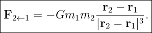
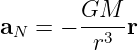
Newton’s law of universal gravitation is often presented in a textbook as a finished formula,

|----------------------------| | --r2 −-r1 | |F2←1 = − Gm1m2 |r2 − r1|3 .| -----------------------------

(1)

A more interesting question is: how could observations tell us that gravity has this form?

This article reconstructs that logic twice. First, it follows the historical chain from Tycho Brahe’s precise observations, through Kepler’s empirical orbital rules, to Newton’s dynamical interpretation. Second, it repeats several of the key tests with modern Solar-System data from NASA and the Jet Propulsion Laboratory (JPL).

The word “prove” must be used carefully in experimental physics. Observations do not prove a physical law in the deductive sense of a mathematical theorem. They test the law against nature over a specified domain and precision. Modern gravity models are also not purely Newtonian: high-precision planetary ephemerides include many-body perturbations, nonspherical gravity, relativistic corrections, observational biases, and other effects [8, 7]. What we can test very strongly is that Newton’s central inverse-square law is the dominant Solar-System gravitational law and that modern observations recover its characteristic signatures.

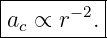
The main empirical chain studied here is

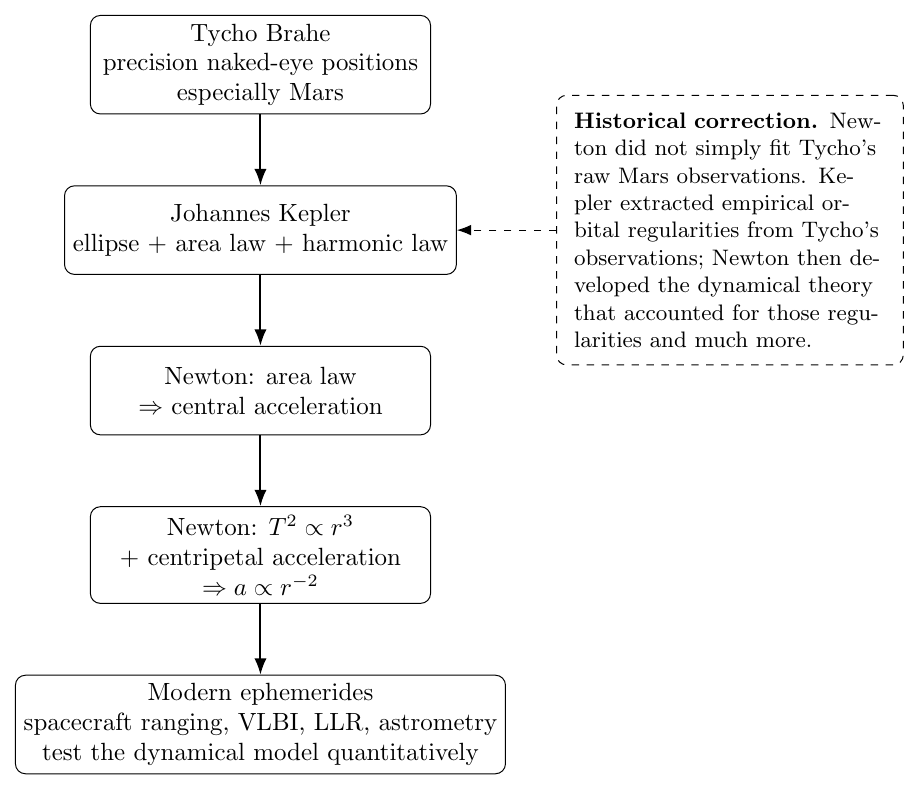
|----------------------------------------------------| observed motion −→ central acceleration −→ T 2 ∝ a3| | −2 | -----−→--|a| ∝-r--−-→--GM---from--the-orbital-scale-----

(2)

Figure 1. The historical and modern logic. Tycho’s observations fed Kepler’s empirical astronomy; Newton transformed orbital regularities into a dynamical theory. Modern ephemerides test a much richer dynamical model against substantially more precise observations.

1. The historical path: Tycho, Kepler, and Newton

1.1 Tycho Brahe supplied precision observations, not Newton’s force law

Tycho Brahe assembled an unusually precise naked-eye observational record of planetary positions during the late sixteenth century. Mars was especially important because its relatively large orbital eccentricity makes departures from uniform circular motion easier to detect than for nearly circular planets.

After working with Tycho in Prague and succeeding him as Imperial Mathematician, Johannes Kepler used Tycho’s observations extensively in the Astronomia Nova of 1609. Kepler tested a traditional circular-orbit construction against Mars observations and found an approximately eight-arcminute discrepancy that he regarded as too large to dismiss given the quality of Tycho’s observations. This failure became part of the route to a new orbital description [2, 1].

The historical chain is therefore more precise than the common statement that “Newton used Tycho Brahe’s data.” Newton did not simply perform a force-law fit to Tycho’s raw Mars measurements. Kepler first transformed observations into empirical regularities about planetary motion. Newton later supplied a dynamical framework in which those regularities, together with observations of planetary satellites and other phenomena, could be understood as consequences of centripetal gravitational forces [4, 3].

1.2 Kepler’s observational regularities

In modern language, three Keplerian statements became particularly important:

planets approximately follow ellipses with the Sun at one focus;
the radius vector from the Sun sweeps equal areas in equal times;
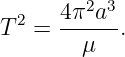
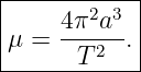
the orbital periods and semimajor axes approximately satisfy
$2 3 T ∝ a .$ (3)

The first two emerged from Kepler’s Mars work; the harmonic relation was published later in Harmonices Mundi. Historically, Newton treated such astronomical “phenomena” as high-quality approximations rather than exact statements about an isolated two-body universe [4].

1.3 From the area law to a central force

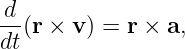
CM04 derived the differential-area relation

dA- = h, h = |r × v |. dt 2

(4)

Constant areal velocity means

dh- dt = 0.

(5)

Because

d --(r × v) = r × a, dt

(6)

we obtain

|----------| |r × a = 0.| ------------

(7)

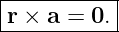
Thus the acceleration must be parallel or antiparallel to the radius vector. The area law is therefore evidence that the dominant acceleration is central: it points along the line joining the planet and the Sun.

This result does not yet tell us how the magnitude varies with distance. For that, the period-distance relation supplies the next clue.

1.4 Kepler’s harmonic law plus circular dynamics gives the inverse square

For uniform circular motion of radius r and period T,

2πr- v = T .

(8)

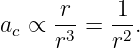
The centripetal acceleration is

a_c	=	(9)
	= ²	(10)
	= .	(11)

If the orbital data obey

T2 ∝ r3,

(12)

then

r 1 ac ∝ r3 = r2.

(13)

Therefore

|-----−-2-| ac-∝-r--.--

(14)

This is the elementary observational route to an inverse-square acceleration. Newton’s actual reasoning was richer than this nearly-circular approximation. In the Principia, he connected the area rule to centripetal force, considered satellite systems as well as planets, and related the detailed absence or presence of apsidal motion to the force law [4, 3].

2. Turn Newton’s inverse square into a parameter the data can estimate

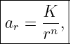
Instead of assuming an inverse-square law from the start, suppose the radial acceleration magnitude follows a generalized power law

|--------| ar = K-,| ------rn--

(15)

where K and n are unknown. Newtonian point-mass gravity corresponds to

n = 2, K = GM.

(16)

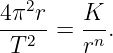
For a circular orbit,

4π2r- K-- T 2 = rn .

(17)

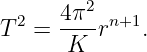
Rearranging,

4π2 T2 = ----rn+1. K

(18)

Take logarithms:

( 4π2 ) 2lnT = ln ---- + (n + 1) ln r. K

(19)

Equivalently,

|-----------------| ln T = α + β lnr, | ------------------

(20)

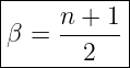
with

|----------| | n-+-1-| |β = 2 | ------------

(21)

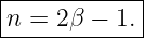
and hence

|------------| -n-=-2β-−--1.|

(22)

This is useful experimentally. We can fit the observed slope β in log–log space and let the orbital data estimate the force-law exponent n.

For elliptical Keplerian orbits the correct characteristic radius is the semimajor axis a, and Newtonian two-body dynamics gives exactly

2 4π2- 3 T = μ a , μ = G(M + m ).

(23)

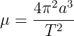
For a planet with m ≪ M_⊙, μ ≃ GM_⊙.

3. Modern data used in this article

The first data set contains the eight planets from Mercury through Neptune. The accompanying CSV records J2000-style semimajor axes and sidereal periods from the NASA planetary fact sheets, together with perihelion/aphelion distances and the corresponding maximum/minimum orbital speeds used in the area-law test. NASA’s fact-sheet notes explain that the compiled values draw on sources including JPL ephemerides, astronomical almanacs, IAU/IAG reports, and current literature; the values are research products rather than a single set of immutable “official” constants [5].

The second data set contains eight regular inner/Galilean moons of Jupiter from JPL’s Planetary Satellite Mean Elements page: Metis, Adrastea, Amalthea, Thebe, Io, Europa, Ganymede, and Callisto. JPL states that these mean elements are precessing ellipses fitted in a least-squares sense to numerically integrated satellite orbits, and warns that accurate ephemeris computation should use horizons rather than the mean-element table [6].


Planet	a (au)	T (days)

Mercury	0.38709893	87.969
Venus	0.72333199	224.701
Earth	1.00000011	365.256
Mars	1.52366231	686.980
Jupiter	5.20336301	4332.589
Saturn	9.53707032	10755.699
Uranus	19.19126393	30685.400
Neptune	30.06896348	60189.018

Table 1. Planetary semimajor axes and sidereal periods used in the log–log fit. The machine-readable values and source URLs are included in planetary_orbit_data.csv.


Jupiter moon	a (km)	T (days)

Metis	128000	0.294779
Adrastea	129000	0.298260
Amalthea	181400	0.499918
Thebe	221900	0.676105
Io	421800	1.762732
Europa	671100	3.525463
Ganymede	1070400	7.155588
Callisto	1882700	16.690440

Table 2. JPL JUP365 mean semimajor axes and orbital periods for eight regular Jovian satellites used in the independent exponent fit [6].

4. Modern test I: does the motion look central?

For a central force,

h = r2𝜃˙= constant.

(24)

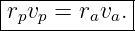
At perihelion and aphelion the radial velocity is zero, so the velocity is transverse. Therefore

h = r v, h = r v . p p p a a a

(25)

A central two-body orbit predicts

|------------| -rpvp =-rava.|

(26)

Using the rounded perihelion/aphelion distances and maximum/minimum speeds published in the NASA fact sheets, define the diagnostic

( ) rpvp- Δh = 100 rava − 1 percent.

(27)

The resulting values are


Planet	Δ_h (percent)

Mercury	−0.01870
Venus	+0.02050
Earth	+0.01119
Mars	−0.00072
Jupiter	+0.05325
Saturn	−0.02948
Uranus	+0.02619
Neptune	−0.09974

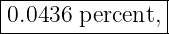
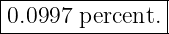
The root-mean-square mismatch is about

|---------------| 0.0436-percent,--

(28)

and the largest absolute mismatch is about

|---------------| 0.0997 percent. | -----------------

(29)

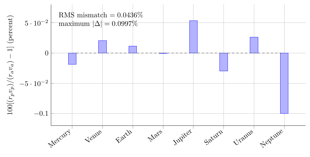
Figure 2. A simple areal-law diagnostic from rounded NASA fact-sheet values. The small residuals should not be interpreted as independent measurement uncertainties; the input values are rounded ephemeris-derived quantities.

The result is not a precision test of angular-momentum conservation, because the tabulated values are rounded and correlated products of orbit determination. It is nonetheless a striking classroom-scale demonstration that modern published orbital quantities obey the central-force signature rv = constant at the apsides to roughly one part in 10³ or better.

5. Modern test II: let the planets estimate the force exponent

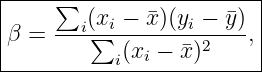
For the eight planets, perform an ordinary least-squares fit

yi = α + βxi, xi = ln ai, yi = ln Ti.

(30)

The fitted slope from the values in Table 1 is

|------------------| -β-=-1.4998265333.--

(31)

The generalized power-law exponent is therefore

n	= 2β − 1	(32)
	= 2(1.4998265333) − 1,	(33)

|------------------| -n-=-1.9996530665.--

(34)

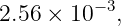
The fit has

|----------------------| -R2-=--0.999999994477.--|

(35)

The formal ordinary-least-squares standard error propagated to n is approximately

SEOLS (n) ≃ 9.10 × 10−5.

(36)

That number is a formal regression error only. It is not a complete experimental uncertainty on the exponent of gravity. The orbital quantities are model-derived, highly correlated, and subject to systematic assumptions that are not represented by an elementary two-column regression.

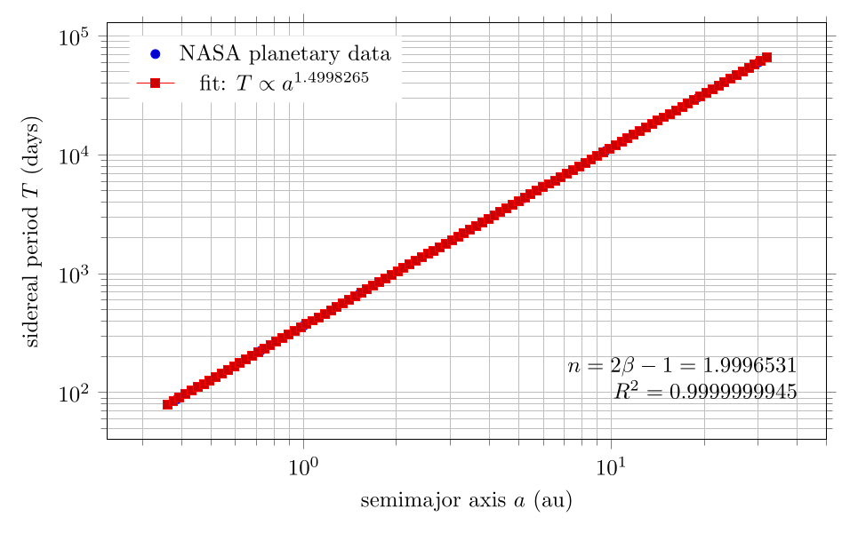
Figure 3. Eight-planet log–log fit. The observed period–semimajor-axis slope is extremely close to 3∕2, corresponding to an inferred central-force exponent extremely close to n = 2.

The scale range is itself notable: the fit spans semimajor axes from about 0.39 au for Mercury to about 30.07 au for Neptune, nearly two orders of magnitude in radius. The leading-order Solar-System relation has the power expected from inverse-square gravity across that entire interval.

6. Modern test III: repeat the exponent test around Jupiter

A strong empirical law should not depend on choosing the Sun as the central body. Newton emphasized satellite systems precisely because the same dynamical logic could be applied around planets [4, 3].

Apply the same regression to JPL’s eight regular Jovian moons in Table 2. The result is

|------------------| β = 1.5001941727 | --J-----------------

(37)

and hence

|------------------------------| -nJ-=-2βJ-−--1 =-2.0003883453.-|

(38)

The fit gives

|--2-------------------| -R-J =-0.999995641062.--|

(39)

The formal OLS standard error of n_J is approximately

−3 2.56 × 10 ,

(40)

again with the important warning that this is not a complete physical uncertainty budget.

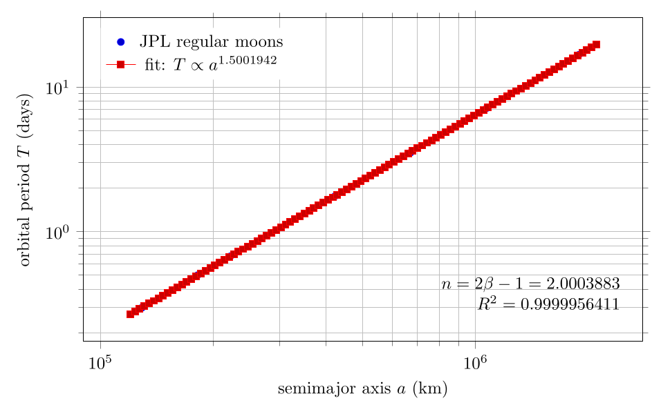
Figure 4. Independent period–radius regression for eight regular satellites of Jupiter. A different central body again gives a power-law exponent very near two.

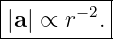
The Sun and Jupiter systems therefore tell the same leading-order story:

|----------| ||a| ∝ r −2. -----------

(41)

This is much closer in spirit to Newton’s claim of universality than a fit to only one planet or one central body.

7. Recover the scale of the law: estimate GM_⊙

The exponent tells us how the acceleration changes with distance. The constant of proportionality tells us the strength of the central gravitational field.

For a Newtonian two-body orbit,

2 3 T2 = 4π--a-. μ

(42)

Therefore

|-----------| | 4π2a3 | μ = ---2-. | ------T------

(43)

As a numerical example, use Venus:

a = 0.72333199 au, T = 224.701 days.

(44)

The International Astronomical union defines

1 au = 149597870700 m

(45)

exactly, and recommends that the solar mass parameter be determined observationally in SI units [9].

Converting units and inserting the Venus values gives

|--------------------------------------| |μ⊙,Venus ≃ 1.327123976 × 1011 km3/s2. | ---------------------------------------

(46)

JPL’s DE440 astrodynamic-parameter value is

|--------------------------------------------| |GM = 1.32712440041279419 × 1011 km3/s2. | -----⊙----------------------------------------

(47)

The simple Venus two-body reconstruction differs by approximately

|------------------------| − 0.320 parts per million.| --------------------------

(48)

This comparison is educational rather than an independent precision experiment. The published semimajor axis and period are themselves products of astronomical orbit determination and modern dynamical modeling. The agreement shows internal consistency of the two-body scale at an impressive level; it should not be advertised as an independent 0.32-ppm measurement of Newtonian gravity.

8. Why modern ephemerides are a much stronger test than these tables

The preceding calculations deliberately use compact published orbital summaries because they expose the physics. Modern Solar-System gravity tests operate at a much deeper level.

JPL’s DE440 and DE441 planetary/lunar ephemerides were produced by fitting numerically integrated trajectories to ground- and space-based observations. The data include spacecraft radio ranging, Very Long Baseline Array measurements, optical astrometry, lunar laser ranging, occultation data, and other observations. For example, DE440 incorporated Juno ranging and VLBA data to improve Jupiter’s orbit and Cassini ranging and VLBA data to improve Saturn’s orbit [8].

Conceptually, modern orbit determination looks like Figure 5.

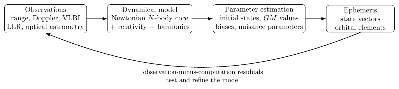
Figure 5. Modern ephemeris construction. Observations are compared with numerically integrated dynamical predictions; parameters are estimated and observation-minus-computation residuals expose inadequacies in the model.

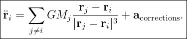
At leading order, the acceleration of body i due to point-mass Newtonian interactions is

|----∑---------r-−-r---------------| ¨ri = GMj --j----i-+ acorrections.| | j⁄=i |rj − ri|3 | ------------------------------------

(49)

The correction term may contain relativistic contributions, nonspherical gravity, asteroid perturbations, tidal effects, and other modeled accelerations appropriate to the data set. The power of the modern test is not that one draws a straight line through eight points; it is that one integrated dynamical model must account simultaneously for enormous collections of heterogeneous observations over long time spans.

9. Newton’s law is extraordinarily successful, but not exact

The inverse-square form

a = − GM--r N r3

(50)

is the dominant weak-field, low-speed gravitational acceleration in the Solar System. It is not the complete modern theory of gravity. General relativity predicts corrections that become measurable in precise planetary and spacecraft data, including relativistic perihelion advance and propagation-time effects. Modern ephemerides therefore do not test “Newton versus data” in isolation; they test a hierarchy of dynamical models in which Newtonian gravity provides the leading term [8].

This distinction illustrates how physical science works. A law can be spectacularly successful within a domain while being recognized as the limiting form of a more general theory.

10. Reproducible calculation with Julia

The accompanying file

newton_modern_data_analysis.jl

reproduces the numerical calculations using only the Julia standard library. It reads

planetary_orbit_data.csv

and

jupiter_regular_moons_data.csv,

performs the two log–log linear regressions, computes

n = 2β − 1,

(51)

checks the apsidal quantity rv, and reconstructs GM_⊙ from the Venus pair (a,T).

For a set of points (x_i,y_i), the code uses the ordinary least-squares slope

|----∑-------------------| |β = ---i(x∑i-−-¯x)(yi −-¯y),| | i(xi − ¯x )2 | --------------------------

(52)

where

xi = ln ri, yi = ln Ti.

(53)

The numerical values printed by the supplied script are recorded in analysis_results.txt. The article’s results were independently cross-checked during preparation. A Julia installation is sufficient to reproduce the calculation; no astronomy package is required because the source data have already been frozen into the supplied CSV files.

10.1 File downloads from the PhysicsLibrary filebox

The reproducibility files used in this article can be attached directly to the PhysicsLibrary object’s filebox. PhysicsLibrary’s manual file-link command is

∖PMlinktofile{anchor text}{filename}.

Once the files have been uploaded to this object’s filebox with the exact filenames shown below, the following links provide direct downloads:

The Julia script and the two CSV files are sufficient to reproduce the numerical tests in this article. The text results file is included as a convenient reference output. The filebox names are intentionally kept simple and should be uploaded without renaming so that the manual links remain valid.

For a higher-fidelity extension, one could query JPL Horizons or use Astropy/Astroquery to obtain epoch-specific state vectors, numerically differentiate or fit trajectories, and compare observation-based residuals with Newtonian and post-Newtonian models. That would move the exercise from an orbital-summary test toward a simplified form of real orbit determination.

11. What has actually been demonstrated?

The modern data used here support four distinct statements:

The small apsidal rv mismatches are consistent with the central-force/constant-areal-velocity structure expected from angular-momentum conservation.
The eight planetary periods and semimajor axes give
$n ≃ 1.99965,$ (54)

when a generalized central force a ∝ r⁻ⁿ is inferred from the period–distance scaling.
An independent fit to eight regular moons of Jupiter gives
$nJ ≃ 2.00039.$ (55)

Thus the same inverse-square behavior appears around a second central body.
The scale relation
$4π2a3- μ = T2$ (56)

recovers the solar gravitational parameter from a simple planetary orbit at a value extremely close to the modern JPL value.

These are not logically independent, raw-observation proofs of Newton’s law: the orbital elements themselves are derived using modern ephemeris models. They are transparent consistency tests that allow a student to reproduce, with modern numbers, the essential observational logic behind Newtonian celestial mechanics.

The most important result is therefore not merely

|------| |n ≈ 2.| --------

(57)

It is the methodological chain

|----------------------------------------------------------| |measure −→ find empirical regularities −→ infer dynamics | | | ---−→--predict-new-motion--−→--compare--with-observation---|

(58)

That chain connects Tycho, Kepler, Newton, and modern spacecraft navigation remarkably directly.

12. Suggested extensions

Several natural computational projects follow from this article:

Replace the tabulated mean elements by JPL Horizons state vectors sampled over time and numerically verify constant areal velocity.
Fit a generalized acceleration law directly to numerically estimated accelerations rather than inferring the exponent through Kepler’s third-law scaling.
Repeat the satellite regression for Saturn, Uranus, or Neptune.
Construct Newtonian N-body and relativistic propagators and compare their residuals against modern ephemeris states.
Use Mercury to investigate why a pure Newtonian ellipse does not remain exactly fixed in inertial space.

These extensions naturally connect this application article to later PhysicsLibrary lessons on perturbation theory, numerical integration, N-body dynamics, and relativistic celestial mechanics.

References

[1] J. Kepler, New Astronomy, translated by W. H. Donahue, Cambridge University Press, Cambridge, 1992. Originally published as Astronomia Nova in 1609.

[2] S. Boner and contributors, “Johannes Kepler,” Stanford Encyclopedia of Philosophy, substantive revision 2025. Stanford Encyclopedia of Philosophy: Johannes Kepler

[3] I. Newton, The Principia: Mathematical Principles of Natural Philosophy, new translation by I. B. Cohen and A. Whitman, University of California Press, Berkeley, 1999. Originally published in 1687.

[4] G. E. Smith, “Newton’s Philosophiae Naturalis Principia Mathematica,” Stanford Encyclopedia of Philosophy. Stanford Encyclopedia of Philosophy: Newton’s Principia

[5] NASA National Space Science Data Center, “Notes on the Fact Sheets,” planetary fact-sheet definitions and data-source notes, accessed 2026. NASA NSSDCA Fact Sheet Notes

[6] Jet Propulsion Laboratory Solar System Dynamics, “Planetary Satellite Mean Elements,” including JUP365 mean elements for Jupiter’s regular satellites, accessed 2026. JPL Planetary Satellite Mean Elements

[7] Jet Propulsion Laboratory Solar System Dynamics, “Astrodynamic Parameters,” DE440 gravitational parameters, accessed 2026. JPL Astrodynamic Parameters

[8] R. S. Park, W. M. Folkner, J. G. Williams, and D. H. Boggs, “The JPL Planetary and Lunar Ephemerides DE440 and DE441,” The Astronomical Journal, vol. 161, article 105, 2021.

[9] International Astronomical Union, Resolution B2, “Re-definition of the astronomical unit of length,” XXVIII General Assembly, 2012. IAU 2012 resolutions

[10] J. M. A. Danby, Fundamentals of Celestial Mechanics, 2nd ed., Willmann-Bell, Richmond, 1988.

[11] C. D. Murray and S. F. Dermott, Solar System Dynamics, Cambridge University Press, Cambridge, 1999.

"Testing Newton's Law of Gravitation" is owned by bloftin.
(view preamble)

Testing Newton's Law of Gravitation