Strapdown Inertial Navigation Examples: Vectors, Frames, and Direction Cosine Matrices
This companion to INS01 develops the coordinate-frame machinery through explicit calculations.
The emphasis is not on memorizing rotation matrices. Each exercise asks the reader to connect the
matrix algebra back to the geometry of basis vectors and to the passive transformation
convention
The exercises are stated first so that the article can be used as a self-study problem set. Complete
worked solutions follow in the second half.
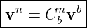
The examples use the same conventions as INS01: body axes are forward–right–down, the local
navigation frame is north–east–down (NED), and a matrix Cbn converts components resolved
in frame b into components resolved in frame n. These conventions are standard in
inertial-navigation treatments such as Titterton and Weston [1], Groves [2], and Jekeli
[3].
1 Exercises
Exercise 1: One vector, two coordinate frames
In a horizontal plane, let the body frame b be rotated counterclockwise by
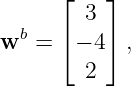
relative to the navigation frame n. A physical vector has body-frame coordinates
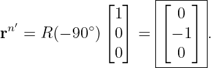
- Construct the passive coordinate transformation Cbn.
- Compute vn.
- Verify that the vector magnitude is unchanged.
- Explain geometrically why the coordinate numbers change even though the physical
vector does not.
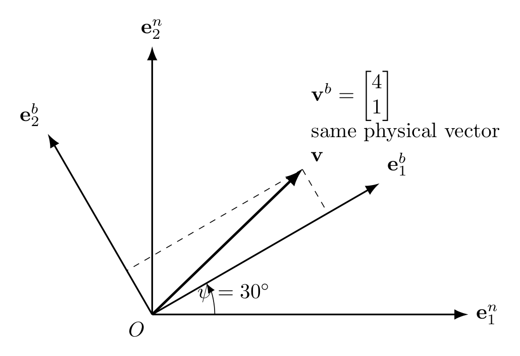
Figure. The same physical vector resolved in two planar frames. The body axes are
rotated by 30∘ relative to the navigation axes.
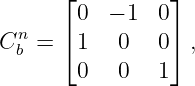
Exercise 2: Construct a DCM directly from basis vectors
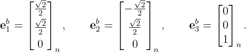
The body basis vectors are given in navigation coordinates by
- Construct Cbn directly from the basis vectors.
- Interpret the first column physically.
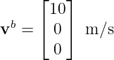
- Transform the body-frame velocity
into NED coordinates.
- State the vehicle heading implied by this result.
Exercise 3: Orthogonality, inverse, and round trip
Using the DCM from Exercise 2:
- Calculate (Cbn)T C
bn.
- Calculate det Cbn.
- Write Cnb without performing a general matrix inversion.
- Starting from
transform to n and then back to b. Verify that the original coordinate column is
recovered.
Exercise 4: Composition and matrix order
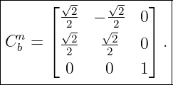
Let frame b be rotated by +25∘ about Down relative to n, and let frame a be rotated by −40∘
about the same axis relative to b.
- Write Cbn and C
ab.
- Form the direct transformation Can.
- What single planar rotation angle does Can represent?
- Transform
into navigation coordinates.
- Explain why Can = C
bnC
ab rather than C
abC
bn.
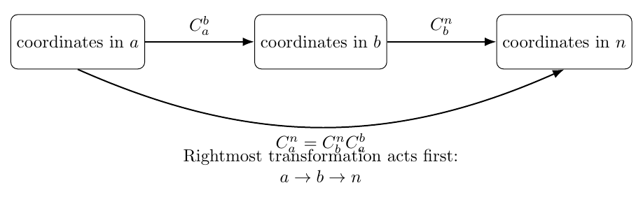
Figure. Coordinate transformations compose by following the frame labels from right to
left.
Exercise 5: Active rotation versus passive coordinate transformation
A vector initially has navigation coordinates
Consider a positive 90∘ rotation about the third axis.
- Actively rotate the physical vector by +90∘ while keeping the navigation axes fixed.
What are the new coordinates?
- Instead keep the physical vector fixed and rotate the coordinate axes by +90∘. What
are the coordinates in the rotated frame?
- Explain why the two matrices have opposite signs in the off-diagonal terms even though
the same angle 90∘ appears in both descriptions.
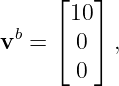
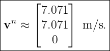
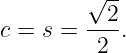
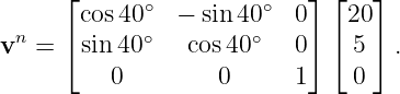
Exercise 6: Body-frame velocity resolved in NED
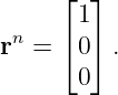
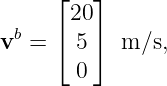
A level vehicle has heading
east of north. Its body-frame velocity is
where the first component is forward and the second is rightward.
- Construct the level-heading DCM Cbn.
- Compute vN, vE, and vD.
- Verify the horizontal speed using both frames.
- Interpret physically why a positive rightward body velocity contributes both north and
east components for this heading.
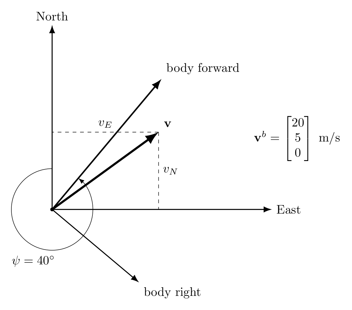
Figure. A level vehicle at 40∘ heading. Body-forward and body-right velocity components
must both be projected onto North and East.
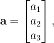
Exercise 7: The skew-symmetric cross-product matrix
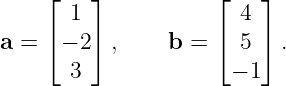
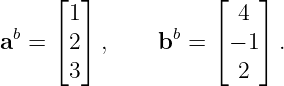
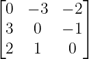
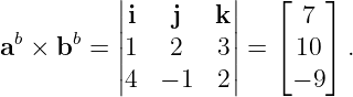
Let
- Construct [a]×.
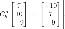
- Compute [a]×b.
- Verify directly that the result equals a × b.
- Verify that [a]×T = −[a]
×.
- Show that aT [a]
×b = 0 and explain the geometry.
Exercise 8: Cross products are geometric and therefore frame consistent
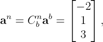
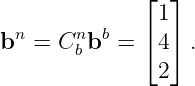
Let
which represents a 90∘ body-to-navigation heading transformation. Let
Compute the cross product in two ways:
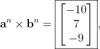
- First evaluate ab × bb in frame b, then transform the result to n.
- Transform a and b separately to frame n, then calculate an × bn.
- Verify that the two answers agree.
- Use the numerical result to illustrate
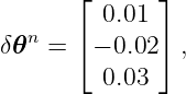
Exercise 9: First-order small angle DCM
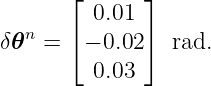
Let the small rotation vector be
- Construct [δ𝜃n]
×.
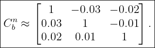
- Form the first-order approximation
- Show symbolically why this approximation is orthogonal to first order.
- For the numerical values above, evaluate (Cbn)T C
bn − I and explain why the residual is
second order rather than zero.
- Explain why repeated use of a first-order matrix without re-orthogonalization
would eventually cause an implemented attitude matrix to drift away from a true
DCM.
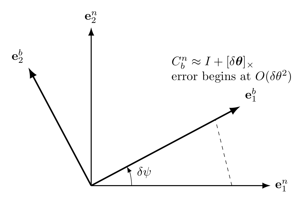
Figure. A small attitude change is represented to first order by I + [δ𝜃]×. Orthogonality
errors appear only at second order.
Exercise 10: Debugging a matrix that looks almost like a DCM
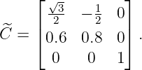
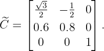
Suppose software reports the matrix
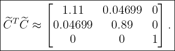
- Evaluate CT C.
- Evaluate det C.
- Is the matrix a valid DCM? Explain which test is decisive.
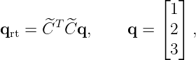
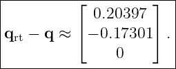
- Apply the round-trip operation
and quantify the failure to recover q.
- Explain why checking only whether the determinant is “close to one” is not sufficient for
validating a numerical attitude matrix.
2 Worked solutions
2.1 Solution 1: One vector, two coordinate frames
For a body frame rotated counterclockwise by ψ relative to n, the body basis vectors resolved in
navigation coordinates are
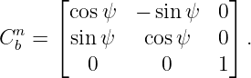
Therefore the passive body-to-navigation DCM is
With ψ = 30∘,
Hence
| vn | = C
bnvb | (16)
|
| = ![[ √- ]
-3- − 1
2 √ 2
12 -23](https://images.physicslibrary.org/cache/objects/1345/make4ht/StrapdownInertialNavigationExamplesVectorsFramesAndDirectionCosineMatrices21x.png) ![[ ]
4
1](https://images.physicslibrary.org/cache/objects/1345/make4ht/StrapdownInertialNavigationExamplesVectorsFramesAndDirectionCosineMatrices22x.png) | (17)
|
| = ![[ √ -- 1 ]
2 3 −√ 2
2 + --3
2](https://images.physicslibrary.org/cache/objects/1345/make4ht/StrapdownInertialNavigationExamplesVectorsFramesAndDirectionCosineMatrices23x.png) . . | (18) |
Numerically,
The body-frame magnitude is
The navigation-frame magnitude is
| ∥vn∥2 | = 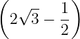 2 + 2 + 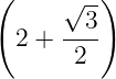 2 2 | (21)
|
| = 17. | (22) |
Thus
The numbers changed because they are projections onto different basis vectors. The geometric
arrow in space did not change.
2.2 Solution 2: Construct a DCM directly from basis vectors
For a passive DCM, the columns of Cbn are the body basis vectors resolved in navigation
coordinates. Therefore
The first column says that the body forward axis has equal North and East components.
Geometrically, body forward points 45∘ east of north.
For
we obtain
| vn | = C
bnvb | (26)
|
| =  m/s. m/s. | (27) |
Numerically,
Thus the implied heading is
2.3 Solution 3: Orthogonality, inverse, and round trip
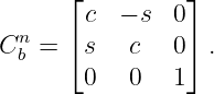
Let
Then
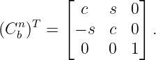
Its transpose is
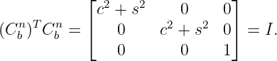
Multiplication gives
Therefore
The determinant is
so this is a proper orthogonal matrix.
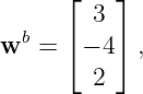
For any vector, including
the round trip is
| wrtb | = C
nbC
bnwb | (37)
|
| = (Cbn)T C
bnwb | (38)
|
| = Iwb | (39)
|
| =  . . | (40) |
This round-trip property is a useful numerical unit test for implemented attitude matrices.
2.4 Solution 4: Composition and matrix order
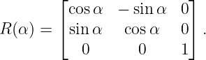
For a positive planar rotation α,
Hence
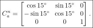
The direct transformation is
Because both rotations are about the same axis,
Thus
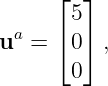
For
| un | = C
anua | (47)
|
| = 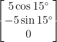 | (48)
|
| ≈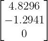 . . | (49) |
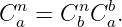
The matrix order follows the coordinate chain:
The rightmost matrix acts first. Reading the frame labels from right to left gives
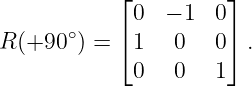
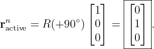
2.5 Solution 5: Active rotation versus passive coordinate transformation
For an active positive 90∘ rotation of the physical vector while the axes remain fixed,
Therefore
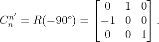
Now hold the physical vector fixed and rotate the coordinate axes by +90∘. Coordinates must then
rotate by the inverse transformation:
Thus
The sign reversal is the essence of the active/passive distinction. Actively rotating a vector by +𝜃
relative to fixed axes is equivalent, at the level of coordinates, to holding the vector fixed and
rotating the axes by −𝜃.
2.6 Solution 6: Body-frame velocity resolved in NED
For a level vehicle with heading ψ, body Down is aligned with navigation Down, so
At ψ = 40∘,
Therefore
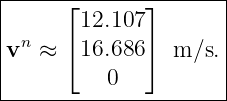
| vN | = 20 cos 40∘− 5 sin 40∘ ≈ 12.107 m/s, | (58)
|
| vE | = 20 sin 40∘ + 5 cos 40∘ ≈ 16.686 m/s, | (59)
|
| vD | = 0. | (60) |
Thus
In body coordinates,
In navigation coordinates,
as required by norm preservation.
The rightward body component is not aligned with East unless the vehicle points exactly North.
At a 40∘ heading, both body-forward and body-right axes have projections onto North and East, so
each body component contributes to both navigation components.
2.7 Solution 7: The skew-symmetric cross-product matrix
For
the cross-product matrix is
Therefore
Multiplying by b,
Direct evaluation of a × b gives the same result.
The transpose is
so the matrix is skew symmetric.
Finally,
The cross product is perpendicular to a, so its dot product with a must vanish.
2.8 Solution 8: Cross products are frame consistent
First calculate the body-frame cross product:
Transforming this result to n gives
Now transform the vectors separately:
and
Their navigation-frame cross product is
which agrees exactly.
Thus
In matrix form this geometric invariance becomes
2.9 Solution 9: First-order small angle DCM
For
the skew matrix is
Hence the first-order DCM is
Let
Because ST = −S,
| (I + S)T (I + S) | = (I − S)(I + S) | (82)
|
| = I − S2. | (83) |
Since every entry of S2 is quadratic in the small angles,
For the numerical vector,
These residuals are of order 10−3, consistent with products of angles of order 10−2 rad.
The first-order matrix is therefore suitable as a local approximation, but it is not an exact element
of SO(3). Repeated multiplication without a proper finite-rotation update or re-orthogonalization
would accumulate norm and orthogonality errors. This motivates the finite attitude-propagation
methods introduced later in the INS series.
2.10 Solution 10: Debugging a matrix that looks almost like a DCM
The reported matrix is
Direct multiplication gives
This is not the identity matrix. The columns are neither perfectly unit length nor mutually
orthogonal.
The determinant is
| det C | =  (0.8) − (0.8) − (0.6) (0.6) | (88)
|
| ≈ 0.99282. | (89) |
That number is fairly close to one, but the matrix still fails the orthogonality test. Therefore
For
the round trip gives
| qrt | = CT Cq | (92)
|
| ≈ . . | (93) |
The error is therefore
This example demonstrates why determinant checking alone is insufficient. A valid DCM must
satisfy all of the defining rotation-matrix properties, especially
and
In practical strapdown software, orthogonality residuals, determinant error, norm preservation, and
round-trip tests provide complementary diagnostics.
3 What these exercises prepare us for
The matrix manipulations in this article are not isolated linear-algebra exercises. They are the
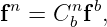
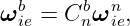
algebraic foundation of the strapdown mechanization. Later we will repeatedly use expressions
such as
and
INS02 adds the missing ingredient: the bases themselves rotate with time. Differentiating a vector
described in a rotating basis will introduce the transport theorem and, after a second
differentiation, the Coriolis, centrifugal, and Euler acceleration terms.
4 Summary
The worked examples reinforce several rules that should become automatic before continuing the
series:
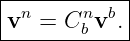
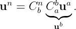
means “take components from b to n.” The columns of Cbn are the body basis vectors resolved in
navigation coordinates. A valid DCM satisfies
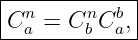
Coordinate transformations compose according to matching frame labels,
and cross products transform consistently because they are geometric operations:
Finally, the small angle approximation
is orthogonal only to first order. That distinction becomes important when attitude is propagated
repeatedly from gyroscope measurements.
References
[1] David H. Titterton and John L. Weston, Strapdown Inertial Navigation Technology,
2nd ed., Institution of Electrical Engineers, 2004.
[2] Paul D. Groves, Principles of GNSS, Inertial, and Multisensor Integrated Navigation
Systems, 2nd ed., Artech House, 2013.
[3] Christopher Jekeli, Inertial Navigation Systems with Geodetic Applications, Walter
de Gruyter, 2001.
[4] Malcolm D. Shuster, “A Survey of Attitude Representations,” The Journal of the
Astronautical Sciences, Vol. 41, No. 4, pp. 439–517, 1993.
[5] F. Landis Markley and John L. Crassidis, Fundamentals of Spacecraft Attitude
Determination and Control, Springer, 2014.

![[parent]](https://images.physicslibrary.org/images/uparrow.png)

![[4]
vb = .
1](https://images.physicslibrary.org/cache/objects/1345/make4ht/StrapdownInertialNavigationExamplesVectorsFramesAndDirectionCosineMatrices2x.png)


![[Cnab] = Cn [ab] Cb .
b × b × n](https://images.physicslibrary.org/cache/objects/1345/make4ht/StrapdownInertialNavigationExamplesVectorsFramesAndDirectionCosineMatrices13x.png)
![Cnb ≈ I + [δ𝜃n]×.](https://images.physicslibrary.org/cache/objects/1345/make4ht/StrapdownInertialNavigationExamplesVectorsFramesAndDirectionCosineMatrices15x.png)
![[ ] [ ]
eb= cosψ , eb = − sin ψ .
1 sinψ n 2 cos ψ n](https://images.physicslibrary.org/cache/objects/1345/make4ht/StrapdownInertialNavigationExamplesVectorsFramesAndDirectionCosineMatrices18x.png)
![|-----[--------------]--|
| n cos ψ − sinψ |
C b = sinψ cosψ . |
-------------------------](https://images.physicslibrary.org/cache/objects/1345/make4ht/StrapdownInertialNavigationExamplesVectorsFramesAndDirectionCosineMatrices19x.png)
![[√ - ]
n -23 − 12
C b = 1 √3- .
2 2](https://images.physicslibrary.org/cache/objects/1345/make4ht/StrapdownInertialNavigationExamplesVectorsFramesAndDirectionCosineMatrices20x.png)
![|----------------|
| [2.9641] |
|vn ≈ .|
--------2.8660---](https://images.physicslibrary.org/cache/objects/1345/make4ht/StrapdownInertialNavigationExamplesVectorsFramesAndDirectionCosineMatrices24x.png)










![⌊ 0 − a a ⌋
⌈ 3 2 ⌉
[a]× = a3 0 − a1 .
− a2 a1 0](https://images.physicslibrary.org/cache/objects/1345/make4ht/StrapdownInertialNavigationExamplesVectorsFramesAndDirectionCosineMatrices62x.png)
![|-------⌊-----------⌋--|
| 0 − 3 − 2 |
|[a ] = ⌈3 0 − 1⌉ .|
| × |
---------2---1----0----|](https://images.physicslibrary.org/cache/objects/1345/make4ht/StrapdownInertialNavigationExamplesVectorsFramesAndDirectionCosineMatrices63x.png)


![[a]T× = − [a ]×,](https://images.physicslibrary.org/cache/objects/1345/make4ht/StrapdownInertialNavigationExamplesVectorsFramesAndDirectionCosineMatrices67x.png)
![aT[a] b = a ⋅ (a × b ) = 0.
×](https://images.physicslibrary.org/cache/objects/1345/make4ht/StrapdownInertialNavigationExamplesVectorsFramesAndDirectionCosineMatrices68x.png)

![|----------------------|
|[Cnb ab]× = Cnb [ab]×Cbn.
-----------------------](https://images.physicslibrary.org/cache/objects/1345/make4ht/StrapdownInertialNavigationExamplesVectorsFramesAndDirectionCosineMatrices75x.png)
![⌊ ⌋
n 0 − 0.03 − 0.02
[δ𝜃 ]× = ⌈ 0.03 0 − 0.01⌉ .
0.02 0.01 0](https://images.physicslibrary.org/cache/objects/1345/make4ht/StrapdownInertialNavigationExamplesVectorsFramesAndDirectionCosineMatrices77x.png)
![S = [δ𝜃]×.](https://images.physicslibrary.org/cache/objects/1345/make4ht/StrapdownInertialNavigationExamplesVectorsFramesAndDirectionCosineMatrices79x.png)






![ω × v = [ω]×v.](https://images.physicslibrary.org/cache/objects/1345/make4ht/StrapdownInertialNavigationExamplesVectorsFramesAndDirectionCosineMatrices94x.png)

![|--n--b------n--b----b-|
-[Cb a-]×-=-C-b [a-]×C-n.](https://images.physicslibrary.org/cache/objects/1345/make4ht/StrapdownInertialNavigationExamplesVectorsFramesAndDirectionCosineMatrices98x.png)
![|-n-----------n--|
-Cb-≈--I +-[δ𝜃-]×--](https://images.physicslibrary.org/cache/objects/1345/make4ht/StrapdownInertialNavigationExamplesVectorsFramesAndDirectionCosineMatrices99x.png)