First Complete Fourier Series: Square Wave
FS04, FS05, and FS06 derived the machinery for computing Fourier coefficients. We
now use that machinery from beginning to end on a genuinely nonsinusoidal periodic
waveform.
The square wave is an ideal first complete example because it contains several important Fourier
ideas at once:
- the waveform is periodic but not sinusoidal,
- symmetry eliminates entire families of coefficients,
- the surviving coefficients can be evaluated exactly,
- only odd harmonics remain,
- the harmonic amplitudes decrease as 1∕n,
- finite partial sums visibly approach the waveform away from jumps,
- and the behavior near discontinuities previews the Gibbs phenomenon.
We begin on the reference interval [−π,π], then generalize the result to [−L,L] and to a
time-periodic signal of period T.
1 Define the square wave carefully
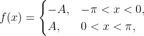
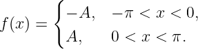
Let A > 0. Define the function over one fundamental interval by
Extend the function periodically so that
This is the odd square wave of amplitude A and period 2π.
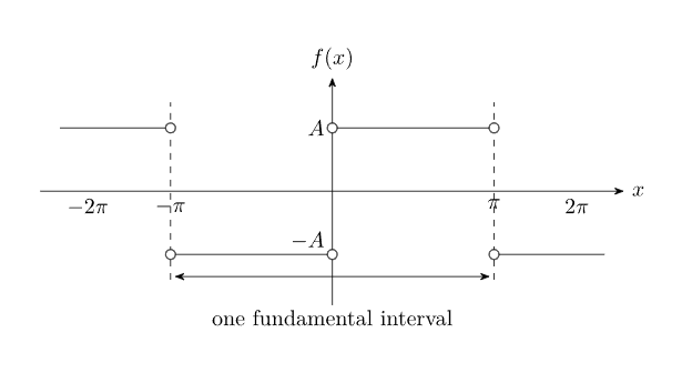
Figure 1. The odd square wave has value −A on the negative half of each period and +A on the
positive half. The isolated jump points do not affect any Fourier coefficient because changing a
function at finitely many points does not change its definite integrals.
What value should we assign at x = 0, x = ±π, and the periodically repeated jump
points?
For coefficient calculations, it does not matter. A definite integral is unchanged if the value of an
integrable function is altered at one isolated point. We may therefore leave the jump values
unspecified for now.
Later convergence articles will distinguish carefully between the value assigned to the original
function and the value approached by its Fourier series at a jump.
2 Start from the complete real Fourier series
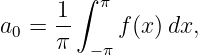
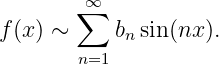
On [−π,π], the real Fourier series has the form
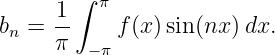
The coefficients derived in FS04 and FS05 are
and
A brute-force calculation could evaluate all three. But before integrating, we should inspect the
waveform.
3 Symmetry first: the square wave is odd
For 0 < x < π,
Then −x lies in (−π, 0), where
Therefore
So the square wave is odd.
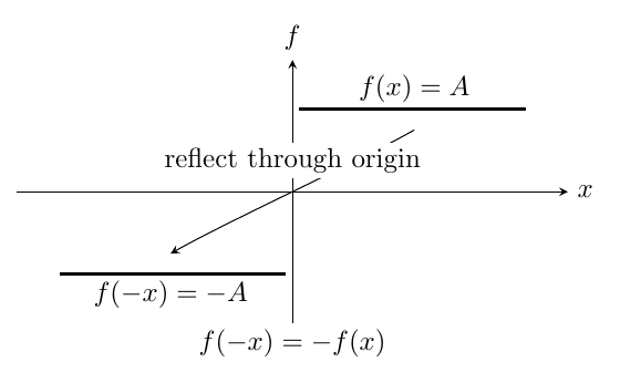
Figure 2. The waveform has origin symmetry. Reflecting a point through the origin changes both
x and the sign of the function value, so f(−x) = −f(x).
This immediately determines two entire coefficient families.
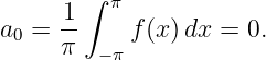
3.1 The constant coefficient vanishes
Because an odd function integrated over a symmetric interval gives zero,
Thus the mean value is
This also makes physical sense: the signal spends equal portions of each period at +A and
−A.
3.2 Every cosine coefficient vanishes
The cosine function is even:
The product of odd f(x) and even cos(nx) is odd. Therefore
for every n ≥ 1.
So before doing any difficult integral, symmetry has reduced the complete series to
This is one of the main practical lessons of Fourier analysis:
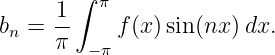
4 Derive the sine coefficients step by step
Start from
Because f(x) changes formula at x = 0, split the integral there:
| bn | =   . | (17) |
Substitute the two constant values of the square wave:
| bn | =   . | (18) |
Factor out A:
| bn | =   . | (19) |
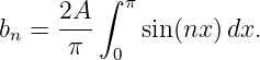
There is a shorter route. Since f(x) is odd and sin(nx) is odd, their product is even:
Therefore
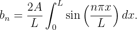
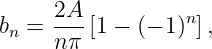
On 0 < x < π, f(x) = A, so
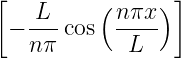
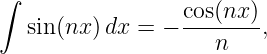
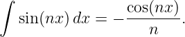
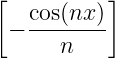
Now integrate:
Hence
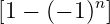
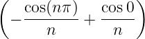
Use
and
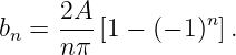
Then
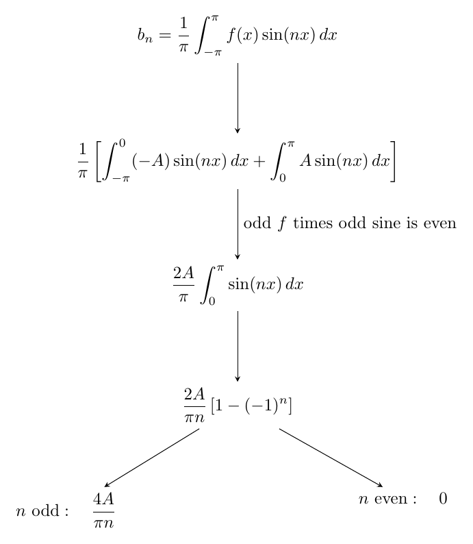
Figure 3. The sine coefficient calculation collapses to one integral over the positive half-period.
The factor 1 − (−1)n then separates odd and even harmonic numbers automatically.
5 Separate odd and even harmonic numbers
Equation (28) contains the entire harmonic-selection rule.
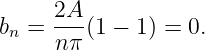
5.1 If the harmonic number is even
Let
Then
Therefore
Every even sine harmonic vanishes.
5.2 If the harmonic number is odd
Let
Then
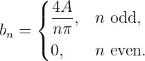
Therefore
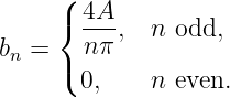
Thus
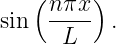
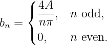
The first few coefficients are therefore
| b1 | =  , | (37)
|
| b2 | = 0, | (38)
|
| b3 | =  , | (39)
|
| b4 | = 0, | (40)
|
| b5 | =  , | (41)
|
| b6 | = 0. | (42) |
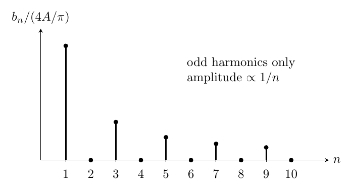
Figure 4. The square-wave sine spectrum contains only odd harmonics. Their magnitudes decrease
as 1∕n, so the third harmonic has one third the first-harmonic amplitude, the fifth has one fifth,
and so on.
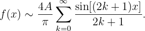
6 Assemble the first complete Fourier series
Substitute the surviving coefficients into the sine-only series:
A compact index uses
so that
This is the first complete nonsinusoidal Fourier series in the FS sequence.
Notice what the series says physically. The square wave is built from ordinary sinusoidal
modes:
- the fundamental sine wave sin x,
- the third harmonic sin 3x,
- the fifth harmonic sin 5x,
- the seventh harmonic sin 7x,
- and all higher odd harmonics.
No even harmonic is required for this particular waveform.
7 Why the coefficient amplitudes decrease inversely with harmonic number
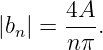
For odd n,
So
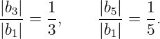
The ratio of the nth odd-harmonic amplitude to the fundamental is
For example,
The slow 1∕n decay is closely connected with the jump discontinuities of the square
wave. Later articles will make the relation between smoothness and spectral decay more
systematic.
8 Half-wave antisymmetry gives a second explanation
The square wave has more structure than ordinary odd symmetry. Shift the waveform by half a
period:
This property is called half-wave antisymmetry.
It explains why even harmonics vanish even before using the explicit square-wave integral.
Consider a generic Fourier integral over one full 2π period and split it into two half-periods. For a
sine coefficient, use the interval [0, 2π]:
| In | = ∫
02πf(x) sin(nx) dx | (51)
|
| = ∫
0πf(x) sin(nx) dx + ∫
π2πf(x) sin(nx) dx. | (52) |
In the second integral let
Then
and
Also,
| sin[n(u + π)] | = sin(nu + nπ) | (56)
|
| = (−1)n sin(nu). | (57) |
Therefore the second half contributes
The two halves combine to give
For even n, the factor is zero.
So half-wave antisymmetry itself suppresses even harmonics. Odd symmetry separately tells us
that this particular phase choice has sine terms rather than cosine terms.
9 Square waves do not always have only sine terms
The result in Equation (45) belongs to the oddly phased square wave of Equation (1).
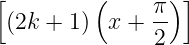
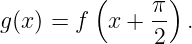
Shift the waveform by π∕2:
This shifted square wave is even rather than odd. Substitute the shift into the sine
series:
For odd integers,
Thus
Therefore the statement
is not generally correct.
The correct statement is that the sine/cosine split depends on the choice of time or spatial origin.
The harmonic frequencies remain the same, but a phase shift redistributes information between
sine and cosine components.
10 Finite partial sums
An infinite Fourier series cannot be drawn directly. We approximate it by keeping finitely many
terms.
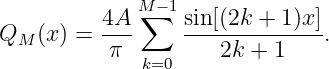
Because only odd harmonics survive, it is convenient to define the partial sum containing the first
M nonzero harmonics:
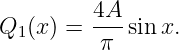
The first partial sum is
The first three nonzero harmonics give
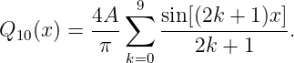
The first ten nonzero harmonics give
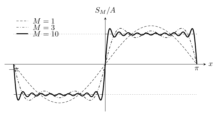
Figure 5. Partial sums built from one, three, and ten nonzero odd harmonics. As more harmonics
are added, the waveform develops flatter plateaus and steeper transitions near the discontinuities.
Every finite QM(x) is continuous because it is a finite sum of continuous sine functions. Yet the
target square wave has jumps. Therefore no finite number of harmonics can reproduce the
discontinuity exactly.
The jump emerges only through the limiting behavior of increasingly many harmonics.
11 What happens exactly at the jump?
At x = 0, every sine term vanishes:
Therefore every finite partial sum satisfies
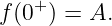
The left and right limits of the square wave are
and
Their midpoint is
So the partial sums already point toward the jump-midpoint rule that will be proved and
formalized later in the convergence sequence.
The same thing happens at x = ±π because
12 Preview of the Gibbs phenomenon
Increasing the number of terms makes the transition region narrower, but the oscillatory overshoot
near a jump does not simply disappear.
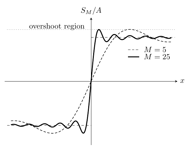
Figure 6. A magnified view near the jump. Adding more odd harmonics squeezes the oscillation
closer to the discontinuity, but a persistent overshoot remains. FS16 will analyze this Gibbs
phenomenon in detail.
For the jump from −A to +A, the jump height is
In the large-partial-sum limit, the first overshoot approaches approximately 8.95% of the jump
height above the upper plateau. Thus the peak approaches roughly
We record this only as a preview. The derivation belongs to FS16.
13 A numerical coefficient table for unit amplitude
Set
Then for odd n,
The first few nonzero values are
| b1 | =  ≈ 1.27324, | (79)
|
| b3 | =  ≈ 0.42441, | (80)
|
| b5 | =  ≈ 0.25465, | (81)
|
| b7 | =  ≈ 0.18189, | (82)
|
| b9 | =  ≈ 0.14147. | (83) |
Notice that the fundamental coefficient is larger than the plateau magnitude A = 1. That does not
mean the square wave itself reaches 1.27324 everywhere. The full waveform results from
interference among all harmonics.
This is an important distinction:
14 A useful special point on the positive plateau
At
the square wave is on its positive plateau, so away from any discontinuity the Fourier series
approaches A.
For the odd harmonics,
sin  | = 1, | (86)
|
sin  | = −1, | (87)
|
sin  | = 1, | (88) |
and so on.
Thus the square-wave series leads to
Cancel A:
Therefore
This is the Leibniz series for π∕4. In this Fourier context it appears naturally by evaluating the
square-wave expansion at a convenient point.
The rigorous justification for substituting into the infinite series will be supplied by the later
convergence results.
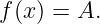
15 Generalize the square wave to an arbitrary symmetric interval
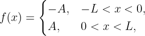
Now define
with periodic extension of period 2L.
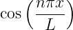
FS06 showed that the basis functions are
and
The waveform is still odd, so
The sine coefficient is
Because the integrand is even,
Integrate:
Therefore
The factor L cancels.
Thus
The coefficient magnitudes are independent of L because stretching the waveform changes the
harmonic wavelengths but not the vertical amplitude ratios.
The general-interval series is
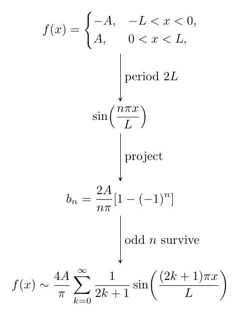
Figure 7. Scaling the period from 2π to 2L changes the harmonic arguments but not the
dimensionless coefficient ratios. The odd square wave still contains only odd harmonics with
amplitudes proportional to 1∕(2k + 1).
16 Time-domain form
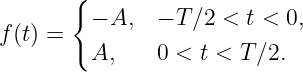
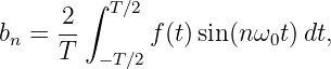
For a signal of period T, use
Define the odd square wave over one centered period by
Then
The frequencies present are
where
16.1 Numerical example
Suppose a square-wave voltage has
and
Then
The first three nonzero harmonic amplitudes are
| b1 | =  V ≈ 6.366 V, | (111)
|
| b3 | =  V ≈ 2.122 V, | (112)
|
| b5 | =  V ≈ 1.273 V. | (113) |
So a three-harmonic approximation is
| f(t) ≈ |  sin(2000πt) +  sin(6000πt) | (114)
|
| +  sin(10000πt). | (115) |
Again, individual coefficient amplitudes can exceed A. Their superposition produces the square-like
waveform.
17 Dimensional check
A Fourier coefficient multiplying sin(nω0t) must have the same units as f because the sine is
dimensionless.
From
the units are
For the square wave,
also has units of amplitude because n and π are dimensionless.
18 Sanity checks on the result
A good Fourier derivation should survive several independent checks.
18.1 Check 1: mean value
The waveform spends equal time at +A and −A, so its mean must vanish. We found
Pass.
18.2 Check 2: parity
An odd waveform should have no cosine terms. We found
Pass.
18.3 Check 3: half-wave antisymmetry
A waveform satisfying
should contain no even harmonics. We found
Pass.
18.4 Check 4: units
Every nonzero coefficient is a dimensionless number times A. Therefore it has the correct
units.
Pass.
18.5 Check 5: period scaling
Replacing [−π,π] by [−L,L] changes the basis argument to
while leaving the amplitude ratios unchanged.
Pass.
19 Common mistakes
19.1 Mistake 1: computing every coefficient before checking parity
For the odd square wave, a0 and all an are known to vanish before integration.
19.2 Mistake 2: forgetting the inverse harmonic factor from integration
Since
the coefficient must contain 1∕n.
19.3 Mistake 3: keeping even harmonics
The factor
is zero for even n.
19.4 Mistake 4: saying every square wave has only sine terms
A phase-shifted square wave can have cosine terms. Sine versus cosine depends on the origin; the
harmonic frequencies are the more invariant feature.
19.5 Mistake 5: expecting a finite sum to contain an exact jump
Every finite trigonometric sum is continuous. A discontinuity appears only through the limit of
increasingly many harmonics.
19.6 Mistake 6: assuming the oscillations near a jump simply vanish
The Gibbs region narrows as more terms are added, but the limiting overshoot remains a fixed
fraction of the jump height.
20 Self-check questions
- Why does a0 vanish for the odd square wave?
- Why does every an vanish?
- Why is f(x) sin(nx) even?
- Starting from the coefficient integral, where does the factor 1∕n enter?
- Why does 1 − (−1)n eliminate even harmonics?
- What is the third-harmonic amplitude relative to the fundamental?
- Why can b1 be larger than A without contradiction?
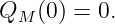
- Why does every finite partial sum satisfy QM(0) = 0?
- What property besides ordinary odd symmetry helps explain the absence of even
harmonics?
- How does the series change when the square wave is stretched from period 2π to period
2L?
- What changes under a phase shift of the square wave, and what does not?
- Why is the overshoot near a jump deferred to a later convergence article?
21 Practice problems
- For A = 2, compute b1, b3, b5, and b7.
- Write the first four nonzero terms of the Fourier series for the odd square wave with
A = 3.
- Show directly from the two piecewise integrals that a0 = 0 without using odd symmetry.
- Show directly that an = 0 by splitting the cosine integral at x = 0.
- Evaluate Q1(π∕2), Q2(π∕2), and Q3(π∕2), where QM contains the first M nonzero odd
harmonics.
- For a square wave on [−4, 4] with amplitude A = 1, write its first three nonzero Fourier
terms.
- A square-wave voltage alternates between −12 V and +12 V at 400 Hz. Find the
frequencies and amplitudes of the first three nonzero harmonics.
- Verify that shifting the odd square wave by π∕2 produces alternating odd cosine
coefficients.
- Use half-wave antisymmetry to prove that even cosine coefficients also vanish for any
waveform satisfying f(x + π) = −f(x), whether or not the waveform is odd.
- Explain why the value assigned to the square wave at x = 0 cannot change any Fourier
coefficient.
22 Summary
For the odd square wave
periodically extended with period 2π, odd symmetry gives
The sine coefficients are
or
Therefore
On the general interval [−L,L],
The square wave therefore establishes the first full connection between a nonsinusoidal periodic
function and its harmonic spectrum.
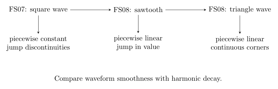
Figure 8. FS07 establishes the complete square-wave calculation. FS08 next compares the
sawtooth and triangle waves, where changes in waveform smoothness lead to different harmonic
structures and decay rates.
References
[1] R. V. Churchill and J. W. Brown, Fourier Series and Boundary Value Problems,
McGraw-Hill.
[2] E. Kreyszig, Advanced Engineering Mathematics, Wiley.
[3] R. Haberman, Applied Partial Differential Equations with Fourier Series and
Boundary Value Problems, Pearson.
[4] G. P. Tolstov, Fourier Series, Dover Publications.

































 sin