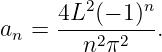
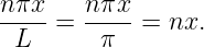
Fourier Series on a General Interval
FS04 and FS05 derived the complete real Fourier coefficient set on the special interval
[−π,π]:
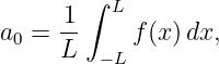
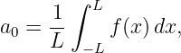
| a0 | =  ∫
−ππf(x) dx, | (1)
|
| an | =  ∫
−ππf(x) cos(nx) dx, | (2)
|
| bn | =  ∫
−ππf(x) sin(nx) dx. | (3) |
Those formulas are not restricted to functions whose natural period happens to be 2π. The interval
[−π,π] is only a convenient dimensionless reference interval.
In this article we stretch or compress that reference interval to
whose total length is
The main goals are to derive, rather than memorize,
and
The corresponding series is
The symbol ∼ is used because the precise conditions under which the infinite series converges to f
are postponed to FS14–FS16.
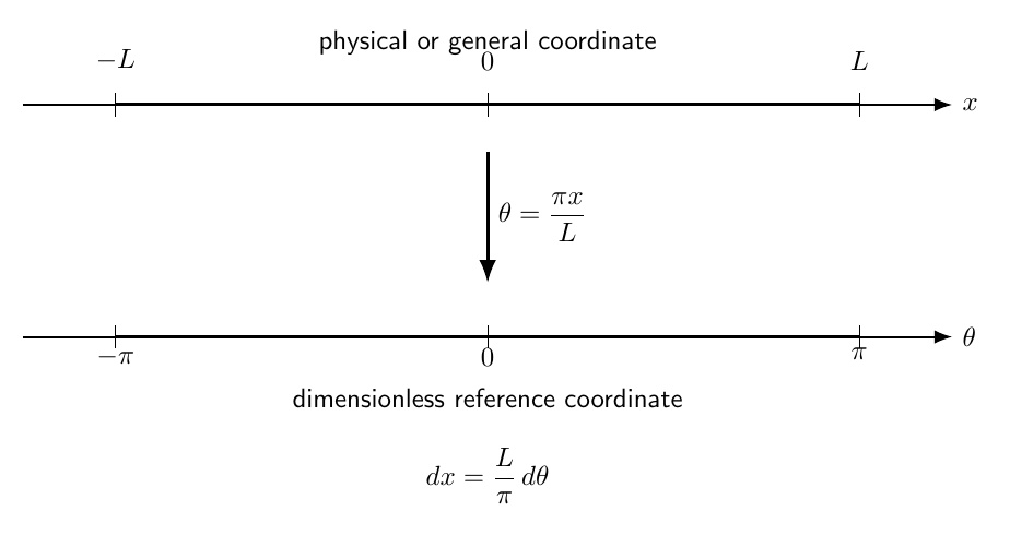
Figure 1. The general interval [−L,L] is mapped to the reference interval [−π,π] by the
dimensionless angle 𝜃 = πx∕L. The endpoints x = −L,0,L map to 𝜃 = −π,0,π.
1 Why the old basis cos(nx) and sin(nx) must change
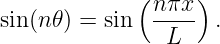
On [−π,π], the full interval has length 2π. The functions
fit an integer number of cycles into that interval.
If the interval changes to [−L,L], the same functions generally no longer fit an integer number of
cycles into one interval of length 2L.
For example, cos x has period 2π. If L = 5, then the interval length is 10, not 2π. There is no
reason for cos x to return to the same phase after moving from one copy of the interval to the
next.
So the harmonic frequencies must scale with L.
2 Deriving the allowed spatial frequencies from periodicity
Consider a cosine of the form
where k is a spatial angular frequency, usually called a Wavenumber.
To repeat after the full interval length 2L, require
for every x.
A cosine returns to the same phase when its argument increases by an integer multiple of 2π.
Therefore require
Divide both sides by 2L:
The smallest positive wavenumber is obtained for n = 1:
Here k0 denotes the fundamental wavenumber. Then
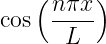
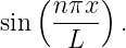
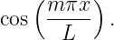
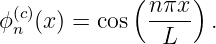
The corresponding basis functions are
and
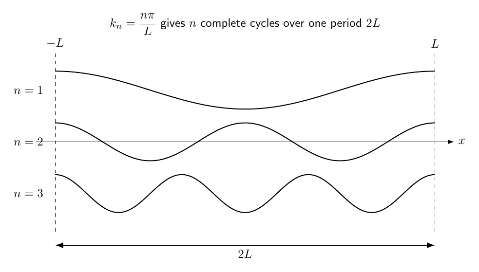
Figure 2. Requiring a phase advance of 2πn across the period 2L gives the discrete wavenumbers
kn = nπ∕L. The nth harmonic completes n cycles over one interval of length 2L.
3 A second derivation by rescaling the coordinate
There is another way to reach the same basis that makes the connection to [−π,π]
explicit.
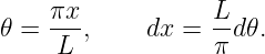
Define the dimensionless variable
When
we obtain
When
we obtain
Thus the map
takes [−L,L] into [−π,π].
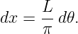
Solve Equation (19) for x:
Differentiate:
The old basis on the reference interval is
Substitute
Then
and
So the periodicity derivation and the coordinate-rescaling derivation agree.
4 Orthogonality must also rescale
The coefficient formulas depend on orthogonality, so we must determine the new inner products on
[−L,L].
Consider two cosine harmonics:
Use
The limits become −π and π, so
| Imn(c) | =  ∫
−ππ cos(n𝜃) cos(m𝜃) d𝜃. | (33) |
FS03 gave
Therefore
| Imn(c) | =  (πδmn) | (35)
|
| = Lδmn. | (36) |
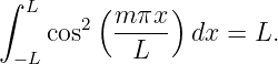
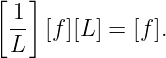
Hence
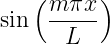
Exactly the same substitution gives
and
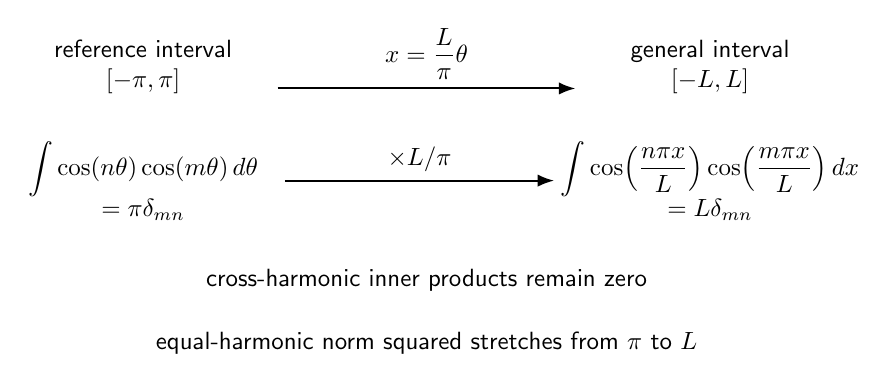
Figure 3. Rescaling the horizontal coordinate stretches the orthogonality interval and also
stretches the basis norms. The zero cross-products remain zero, while the equal-harmonic norm
squared changes from π to L.
5 Norms of the scaled basis functions
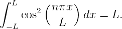
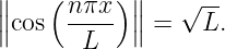
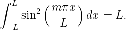
Set m = n in Equation (37):
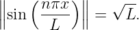
Therefore
Similarly,
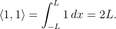
The constant function has norm squared
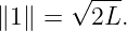
Hence
This already predicts the coefficient normalization:
- nonconstant sine and cosine basis functions have norm squared L, so their projection
coefficients will contain 1∕L;
- the constant basis has norm squared 2L, so the actual constant projection will contain
1∕(2L).
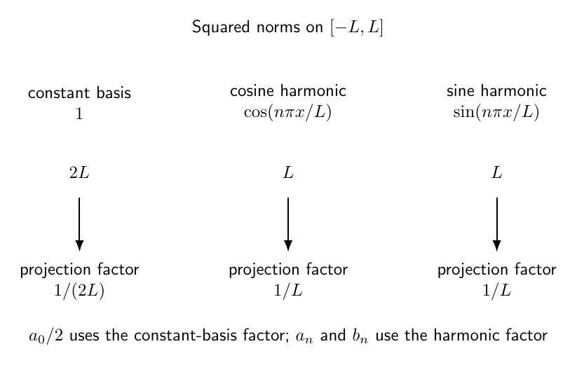
Figure 4. On [−L,L], the constant basis has norm squared 2L, while every nonzero sine or cosine
harmonic has norm squared L. These norms determine the coefficient prefactors.
6 Start with a finite scaled trigonometric expansion
As in FS04 and FS05, begin with a finite expansion so no infinite-series convergence theorem is
needed:
We now extract the coefficients using the same projection operations as before.
7 Derivation of the cosine coefficient on [−L,L]
Choose a positive integer m and multiply Equation (45) by
Then integrate from −L to L:
| ∫
−LLf(x) cos  dx | (47)
|
| =  ∫
−LL cos  dx | (48)
|
| + ∑
n=1Na
n ∫
−LL cos  cos  dx | (49)
|
| + ∑
n=1Nb
n ∫
−LL sin  cos  dx. | (50) |
The first term vanishes because the nonconstant cosine harmonic has zero mean over one complete
period.
The sine-cosine sum vanishes by mixed orthogonality.
Every cosine-cosine term vanishes except the one with n = m.
For that surviving term,
Thus Equation (50) reduces to
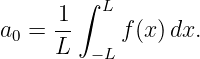
Divide by L:
This is Equation (7).
8 Derivation of the sine coefficient on [−L,L]
Now multiply Equation (45) by
and integrate from −L to L.
The constant term vanishes.
Every cosine-sine term vanishes.
Every sine-sine term with n≠m vanishes.
The surviving equal-harmonic term has norm squared L:
Therefore
Divide by L:
This is Equation (8).
9 Derivation of the constant coefficient
Integrate Equation (45) directly over [−L,L]:
| ∫
−LLf(x) dx | =  ∫
−LL1 dx | (58)
|
| + ∑
n=1Na
n ∫
−LL cos  dx | (59)
|
| + ∑
n=1Nb
n ∫
−LL sin  dx. | (60) |
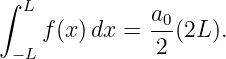
Every nonconstant harmonic integrates to zero over the full period, leaving
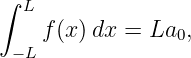
Therefore
and
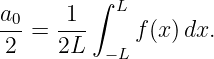
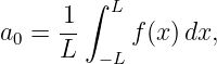
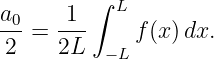
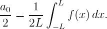
The actual constant term is
Equation (64) is exactly the mean value of f over an interval of total length 2L.
10 The complete Fourier series on [−L,L]
Collecting the results,
with
and
The formulas have exactly the same structure as the [−π,π] formulas. Only the scale of the basis
and the basis norms have changed.
11 Projection interpretation
Define
Its squared norm is
Therefore its projection coefficient is
| cn | = 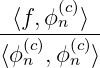 | (71)
|
| =  ∫
−LLf(x) cos  dx | (72)
|
| = an. | (73) |
The same calculation gives bn for the sine basis.
For the constant basis,
Thus all three formulas are one projection rule.
12 Normalized Fourier basis on [−L,L]
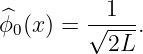
The normalized constant basis function is
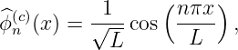
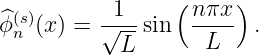
For n ≥ 1, define
and
These satisfy unit norms and mutual orthogonality.
When normalized basis functions are used, the projection coordinates no longer need a
denominator:
and
The numerical coordinate changes, but the projected function does not.
13 Parity shortcuts survive the rescaling
Because [−L,L] is symmetric about zero, all parity arguments from FS05 remain valid.
If f is even, then
for every n, and
Also,
If f is odd, then
and
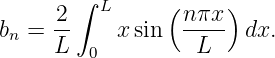
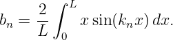
14 Example 1: the odd ramp f(x) = x on [−L,L]
Because f(x) = x is odd,
Only bn remains:
Let
Then
Use integration by parts:
Then
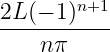
Therefore
| ∫
0Lx sin(k
nx) dx | = 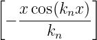 0L +  ∫
0L cos(k
nx) dx. | (91) |
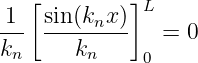
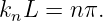
The final integral is
because
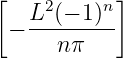
Hence
| ∫
0Lx sin(k
nx) dx | = − | (94)
|
| = − | (95)
|
| = − . | (96) |
Therefore
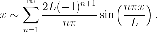
Thus
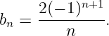
Setting L = π reproduces the FS05 result
15 Example 2: f(x) = x2 on [−L,L]
The function is even, so
The constant coefficient is
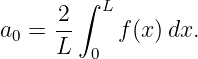
| a0 | =  ∫
0Lx2 dx | (102)
|
| =   0L | (103)
|
| =  . | (104) |
Therefore the mean term is
For n ≥ 1,
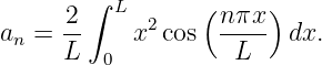
The same two integrations by parts used in FS04 give
Therefore
The coefficient scale is proportional to L2, exactly as dimensional reasoning predicts because x2 has
dimensions of length squared.
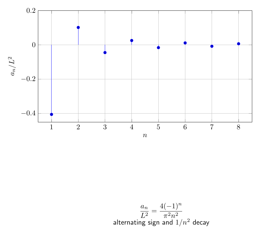
Figure 5. The cosine-series coefficients of x2 on [−L,L] scale as L2∕n2. Changing L changes both
the spatial wavelength of each basis function and the coefficient scale.
16 Example 3: a centered pulse on [−L,L]
Let
This function is even, so
The constant coefficient is
| a0 | =  ∫
−LLf(x) dx | (111)
|
| =  (2Ad) | (112)
|
| =  . | (113) |
Therefore the mean is
For n ≥ 1,
| an | =  ∫
0dA cos  dx | (115)
|
| =  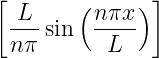 0d | (116)
|
| =  sin  . | (117) |
The coefficient pattern depends only on the dimensionless width ratio
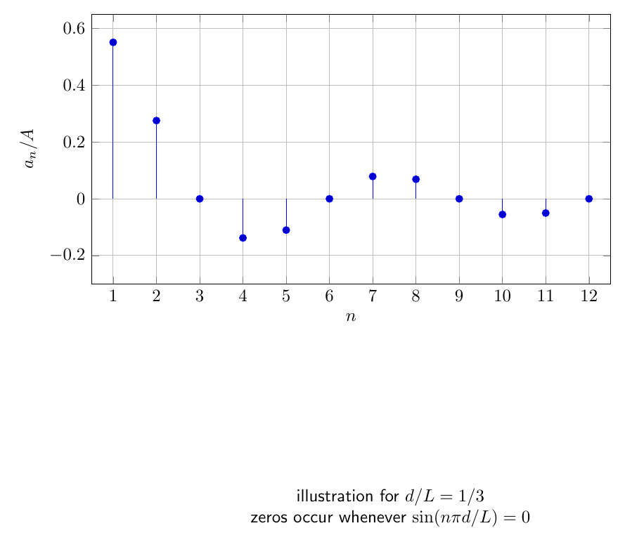
Figure 6. A centered pulse has only cosine harmonics. Its coefficients are proportional to
sin(nπd∕L)∕n, so the spectral pattern is controlled by the fractional half-width d∕L.
17 Recovering the [−π,π] formulas as a special case
Set
Then
Also,
Therefore the general formulas reduce immediately to
and
So FS04 and FS05 are exactly the special case L = π of the present derivation.
18 Time-domain notation: period T
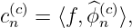
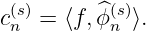
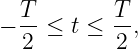
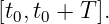
For a time-domain problem, the centered interval is naturally written
where T is the temporal period.
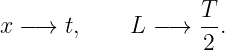
The general-interval formulas are transferred to time by making the mathematical replacements
This is a replacement of interval notation, not an equation between a physical length and a
physical time.
The fundamental angular frequency is therefore
| ω0 | =  | (126)
|
| =  . | (127) |
The harmonic phase becomes
 | =  | (128)
|
| = nω0t. | (129) |
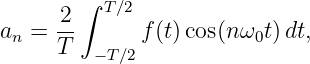
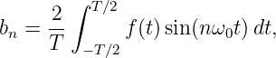
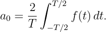
For a T-periodic time signal centered on [−T∕2,T∕2],
with
and
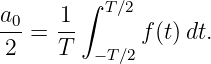
The actual DC term is
19 Spatial wavenumber versus temporal frequency
The same mathematics appears in two common notations.
For a spatially periodic function with period 2L,
and
For a time-periodic function with period T,
and
The basis functions are therefore written as either
or
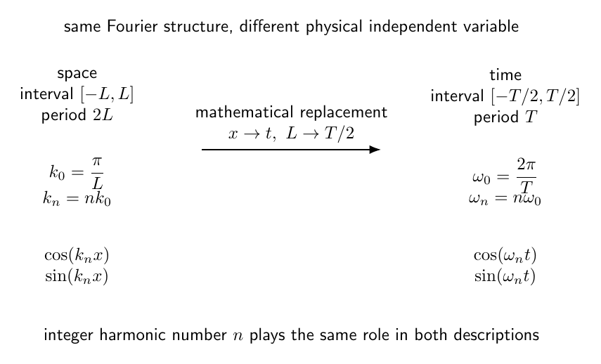
Figure 7. The same harmonic structure appears in space and time. A spatial period 2L gives
k0 = π∕L, while a temporal period T gives ω0 = 2π∕T.
20 Dimensional check
If x has dimensions of length, then
is dimensionless because x∕L is dimensionless.
The trigonometric functions therefore receive dimensionless arguments as required.
The coefficient formula
also has the same dimensions as f:
The same is true for bn and a0.
21 Why the interval must cover one complete period
The formulas above use [−L,L] because that interval has length 2L, which is one complete period
of the chosen basis.
If one integrates over a shorter interval without changing the basis, the cancellation relations can
fail.
The important principle is not the location of the endpoints by itself. The important principle is
that the integration interval span a complete period over which the chosen harmonics are mutually
orthogonal.
Later articles will use intervals such as
or
The basis can be shifted accordingly. The present centered interval is especially convenient because
even/odd parity shortcuts remain available.
22 A practical coefficient workflow on [−L,L]
For a new periodic function on [−L,L]:
- Identify the half-period L.
- Write the fundamental wavenumber
- Write the basis
- Check parity before integrating.
- Compute the mean term
- Compute surviving cosine coefficients.
- Compute surviving sine coefficients.
- Check dimensions.
- Set L = π as a quick consistency test when the example can be compared with an earlier
result.
23 Common mistakes
- Using cos(nx) and sin(nx) on an arbitrary interval without rescaling the argument.
- Writing the fundamental wavenumber as 2π∕L instead of π∕L when the full period is
2L.
- Forgetting that
- Using 1∕π in the coefficient formula after the interval has changed.
- Using 1∕(2L) for an or bn. The 1∕(2L) factor belongs to the actual constant projection
a0∕2.
- Forgetting that the equal-harmonic sine and cosine norm squared is L, not 2L.
- Forgetting to rescale dx when using
- Treating k0 = π∕L as dimensionless when x carries units. A spatial wavenumber has units of
inverse length.
- Confusing the harmonic number n with the physical wavenumber kn.
- Assuming convergence at discontinuities before the convergence theory of FS14–FS16 has
been developed.
24 Practice exercises
- Map [−3, 3] to [−π,π] by defining an appropriate dimensionless variable 𝜃.
- For a function of period 10 m in space, find L, k0, k2, and k5.
- Prove by substitution that
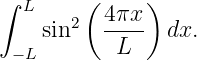
- Evaluate
- Derive the normalized constant basis function on [−L,L].
- Derive the normalized third cosine harmonic on [−L,L].
- For f(x) = x on [−2, 2], calculate b1, b2, and b3.
- For f(x) = x2 on [−2, 2], calculate a
0, a1, and a2.
- For the centered pulse in Equation (109), set A = 3, L = 4, and d = 1. Find the mean and
the first four cosine coefficients.
- Show explicitly that the general ramp coefficient reduces to the FS05 result when
L = π.
- A time signal has period T = 8 s. Find ω0, ω3, and the coefficient prefactor appearing in the
centered-period formulas.
- Explain the difference between the statements “the interval is [−L,L]” and “the period is
2L.”
25 What FS06 has added
The Fourier formulas from FS04 and FS05 were not special formulas tied to the number π. They
were projection formulas written on a convenient reference interval.
The rescaling
shows how the entire construction moves to any centered interval of length 2L.
The basis changes from
to
while the nonconstant basis norm squared changes from π to L.
That one scaling change explains the coefficient prefactor 1∕L.
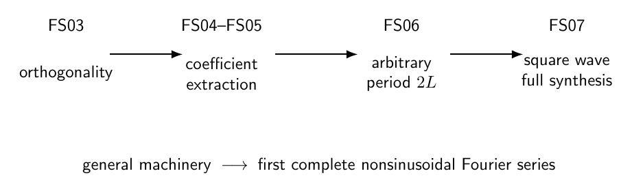
Figure 8. FS06 completes the general coefficient machinery. FS07 will use it on a discontinuous
square wave and watch the harmonic partial sums build an actual nonsinusoidal periodic
waveform.
26 Summary
For a function with period 2L, the fundamental wavenumber is
The harmonic basis is
On [−L,L],
and mixed sine-cosine inner products vanish.
Therefore
and
The actual mean or DC term is
For a time signal centered on [−T∕2,T∕2], replace the mathematical half-interval L by T∕2. The
same structure is then written using
FS07 will now apply these formulas to the first complete nonsinusoidal waveform: the square
wave.
References
[1] R. V. Churchill and J. W. Brown, Fourier Series and Boundary Value Problems,
McGraw-Hill.
[2] E. Kreyszig, Advanced Engineering Mathematics, Wiley.
[3] R. Haberman, Applied Partial Differential Equations with Fourier Series and
Boundary Value Problems, Pearson.
[4] G. B. Arfken, H. J. Weber, and F. E. Harris, Mathematical Methods for Physicists,
Academic Press.