Electromagnetic Waves, Antennas, and RF: Maxwell’s Equations as a Complete System - Exercises
and Complete Worked Solutions
This companion article extends EM15 from recognition of Maxwell’s four equations to active use of
the complete system. The problems emphasize geometric interpretation, dimensional checks,
reconstruction of sources from fields, equivalence of integral and differential forms, constraint
propagation, cylindrical induction problems, and a first plane-wave calculation that prepares the
transition to the electromagnetic wave equation.
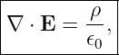
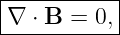
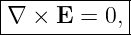
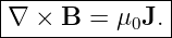
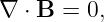
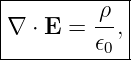
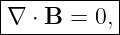
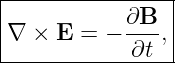
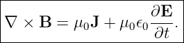
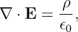
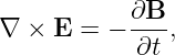
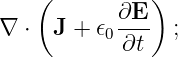
The complete differential system in vacuum with charge density ρ and current density J
is
and
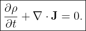
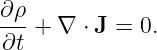
The exercises below should be worked by treating Maxwell’s Equations as one coupled field system
rather than four unrelated formulas [1, 2, 3, 4, 5].
How to use this problem set
Attempt all exercises in Part I before consulting Part II. For every problem, first identify which
Maxwell equation is relevant and whether the geometry suggests a divergence theorem, Stokes
theorem, local differential calculation, or symmetry argument. Keep the following distinctions
explicit:
- divergence versus curl;
- closed surfaces versus closed contours;
- charge density ρ versus current density J;
- conduction current versus displacement-current contribution;
- field constraints versus field-evolution equations;
- source-free vacuum versus field-free space.
Part I: Exercises
Exercise 1: structural map of Maxwell’s equations
For each of the four differential Maxwell equations:
- classify it as a divergence law or curl law;
- identify the corresponding integral theorem used to obtain the integral form;
- state the geometry of the integral form: closed surface or closed contour plus spanning
surface;
- identify the physical source or dynamical quantity appearing on the right-hand side.
Then explain why the two divergence laws are naturally interpreted as constraints while the two
curl laws contain the explicit time coupling that drives field evolution.
Exercise 2: dimensional consistency of the complete system
Verify the dimensions of each Maxwell equation in SI units.
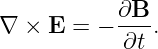
Show explicitly that
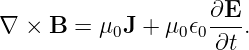
and
Use
Explain why dimensional agreement is a useful but not sufficient test of a field equation.
Exercise 3: an electric field with divergence but no curl
Consider
where α, β, and γ are constants.
Find:
- ∇⋅ E;
- ∇× E;
- the charge density ρ required by Gauss’s Law;
- the condition on α, β, and γ for the region to be charge-free.
If the field is static, state what Faraday’s law implies about ∂B∕∂t.
Exercise 4: a magnetic field with curl but zero divergence
Consider the static magnetic field
where b has units of tesla per meter.
Find:
- ∇⋅ B;
- ∇× B;
- the current density J required by the static Ampere law;
- the direction of that current density.
Explain how this example distinguishes zero magnetic divergence from zero magnetic
field.
Exercise 5: derive integral forms from local equations
Carry out both derivations in detail.
- Starting from
integrate over an arbitrary volume V and derive Gauss’s integral law.
- Starting from
integrate over a fixed surface S and derive Faraday’s integral law.
State exactly where the divergence theorem and Stokes’ theorem are used, and state why a fixed
surface permits the time derivative to be moved outside the surface integral in part
(b).
Exercise 6: cylindrical Faraday induction
A spatially uniform magnetic field points in the +z direction inside a circular cylindrical region of
radius R and is negligible outside that region. The field changes with time:
Assume cylindrical symmetry.
- Use Faraday’s law to derive the induced azimuthal electric field Eϕ(r,t) for r < R.
- Derive Eϕ(r,t) for r > R.
- Show that the two expressions agree at r = R.
- Let
with B0 = 3.0 mT, f = 60 Hz, and R = 4.0 cm. Find the maximum magnitude of Eϕ at
r = 3.0 cm and at r = 10.0 cm.
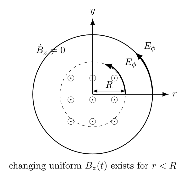
Figure. Circular symmetry converts Faraday’s contour integral into a direct relation
between changing magnetic flux and the induced azimuthal electric field.
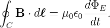
Exercise 7: cylindrical Ampere–Maxwell induction
A spatially uniform electric field points in the +z direction inside a circular region of radius R and
is negligible outside that region:
Assume there is no conduction current through the spanning surface.
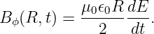
- Use the Ampere–Maxwell law to derive Bϕ(r,t) for r < R.
- Derive Bϕ(r,t) for r > R.
- Show that the two expressions agree at r = R.
- For R = 5.0 cm and
find the magnetic-field magnitude at r = 2.0 cm and r = 10.0 cm.
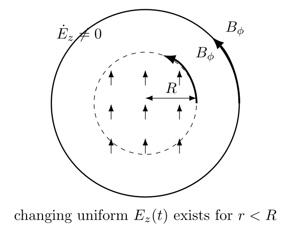
Figure. A changing electric flux produces azimuthal magnetic circulation even when no
conduction current crosses the chosen surface.
Exercise 8: reconstruct the sources from specified fields
Suppose the fields in a region are
and
where a and u are constants with appropriate units.
Use the complete Maxwell system to determine:
- the charge density ρ;
- whether Faraday’s law is satisfied;
- the current density J required by the Ampere–Maxwell equation;
- whether the resulting ρ and J satisfy the continuity equation.
This exercise should be treated as a source-reconstruction problem: the fields are given first, and
the compatible sources must be inferred.
Exercise 9: why the Ampere–Maxwell integral is surface independent
Let S1 and S2 be two different surfaces having the same boundary contour C. Define the effective
current flux through a surface by
Show that
provided charge continuity and Gauss’s electric law hold.
Your proof should:
- combine S1 and S2 into a closed surface;
- use the divergence theorem;
- evaluate
- explain physically why the displacement-current term is necessary.
Exercise 10: propagation of Maxwell’s divergence constraints
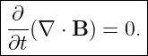
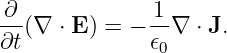
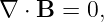
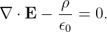
The magnetic divergence law and Gauss’s electric law can be written as constraints on the
instantaneous fields:
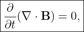
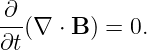
- Take the divergence of Faraday’s law and show that
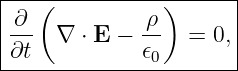
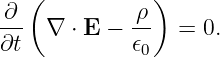
- Take the divergence of the Ampere–Maxwell law, use charge continuity, and show
that
- Explain what these results mean for initial data in an electromagnetic field calculation.
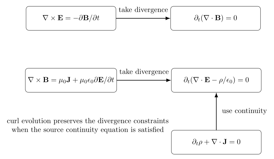
Figure. The curl equations evolve the fields while preserving the divergence constraints,
provided the sources obey local charge conservation.
Exercise 11: plane-wave precursor directly from the curl equations
In source-free vacuum, consider fields of the form
Do not use the electromagnetic wave equation. Use only the two source-free curl equations.
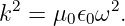
- Apply Faraday’s law and derive a relation among E0, B0, k, and ω.
- Apply the Ampere–Maxwell law and derive a second relation.
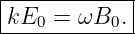
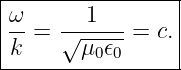
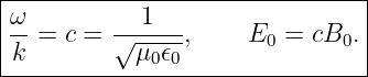
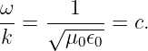
- Combine the two relations to show that
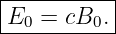
- Show that
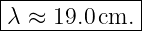
- For f = 1.57542 GHz, compute the vacuum wavelength λ.
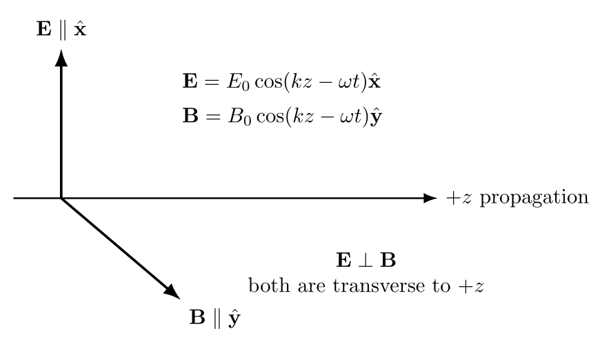
Figure. A transverse plane-wave trial field provides a direct bridge from the coupled curl
equations to the speed c and the amplitude relation E0 = cB0.
Exercise 12: reject a longitudinal vacuum-wave candidate
Consider the proposed source-free vacuum field
- Compute ∇⋅ E.
- Determine whether Gauss’s electric law is satisfied in source-free vacuum for nonzero
k and E0.
- Compute ∇× E and discuss Faraday’s law.
- Explain why satisfying one Maxwell equation is not enough; a candidate field must
satisfy the complete system.
Use this result to motivate why free-space electromagnetic plane waves are transverse rather than
longitudinal.
Exercise 13: recover electrostatics and magnetostatics as limits
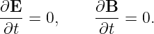
Assume all fields are time independent:
Reduce the complete Maxwell system to its static form.
Then answer:
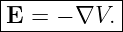
- what does ∇× E = 0 imply locally about an electrostatic potential V ?
- what does the Ampere–Maxwell equation reduce to?
- which two divergence equations remain unchanged?
- why is magnetostatics not obtained by deleting Gauss’s magnetic law?
Exercise 14: source-free does not mean field-free
Determine whether each of the following is a valid source-free, time-independent vacuum solution
of Maxwell’s equations:
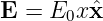
- E = E0x, B = 0;
- E = 0, B = B0z;
- E = E0xx, B = 0;
- E = 0, B = b(−yx + xy).
For each case, evaluate enough divergence and curl quantities to justify the answer. State the
source that would be required when a field is not source-free.
Exercise 15: Julia finite-difference check of divergence and curl
Use central finite differences to numerically verify Exercises 3 and 4 at a point away from any
boundary.
Take
and
Use the point
and finite-difference step
Write a short Julia program that estimates:
- ∇⋅ E;
- ∇× E;
- ∇⋅ B;
- ∇× B.
Compare the numerical values with the exact analytic results.
Part II: Complete Worked Solutions
Solution 1: structural map of Maxwell’s equations
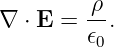
Gauss’s electric law is
It is a divergence law. Integrating over a volume and applying the divergence theorem produces a
closed-surface flux equation. Its source is electric charge density ρ.
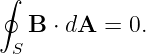
Gauss’s magnetic law is
It is also a divergence law, and the divergence theorem gives the closed-surface result
Its zero right-hand side expresses the absence of magnetic monopole source density in classical
Maxwell theory.
Faraday’s law is
It is a curl law. Stokes’ theorem converts its surface integral into circulation around the
boundary contour. The dynamical quantity on the right is the local time rate of change of
B.
The Ampere–Maxwell law is
It is also a curl law. Its integral form uses a closed contour and spanning surface. Magnetic
circulation is sourced by conduction current density and by changing electric field.
The divergence equations contain no explicit first-order time derivatives of the fields. They
constrain allowable field configurations at each instant. The curl equations explicitly connect time
derivatives of one field to spatial derivatives of the other, so they form the core evolution
coupling.
Solution 2: dimensional consistency of the complete system
Because a spatial derivative contributes one inverse meter,
Also,
so
![[ ]
ρ
--
𝜖0](https://images.physicslibrary.org/cache/objects/1238/make4ht/ElectromagneticWavesMaxwellsEquationsAsACompleteSystemExercisesAndCompleteWorkedSolutions42x.png) | =  | (43)
|
| = V/m2. | (44) |
Thus Gauss’s electric law is dimensionally consistent.
For Faraday’s law,
Using
we obtain
For the magnetic curl equation,
Since
we have
Finally,
so
![[ ]
∂E-
μ0𝜖0∂t](https://images.physicslibrary.org/cache/objects/1238/make4ht/ElectromagneticWavesMaxwellsEquationsAsACompleteSystemExercisesAndCompleteWorkedSolutions51x.png) | =   | (52)
|
| =  | (53)
|
| = T/m. | (54) |
Dimensional agreement is necessary because terms added or equated must share dimensions. It is
not sufficient because an incorrect equation can still be constructed with the correct
units.
Solution 3: an electric field with divergence but no curl
The field is
Its divergence is
| ∇⋅ E | =  + +  + +  | (56)
|
| = α + β + γ. | (57) |
Therefore,
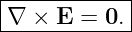
Every cross derivative vanishes, so
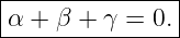
The charge-free condition is therefore
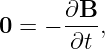
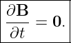
If the field is static, Faraday’s law gives
so
Solution 4: a magnetic field with curl but zero divergence
The field components are
The divergence is
| ∇⋅ B | =  + +  + +  | (64)
|
| = 0. | (65) |
Thus Gauss’s magnetic law is satisfied.
The curl has only a z component:
| (∇× B)z | =  − − | (66)
|
| = b − (−b) | (67)
|
| = 2b. | (68) |
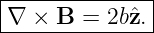
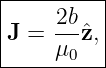
Hence
For a static field, Ampere–Maxwell reduces to
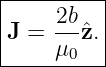
Therefore,
The current density points in the +z direction for positive b. Zero magnetic divergence means
no net magnetic source or sink; it does not require the magnetic field or its curl to
vanish.
Solution 5: derive integral forms from local equations
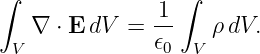
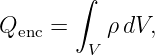
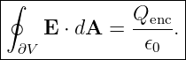
For Gauss’s electric law, integrate over an arbitrary volume V :
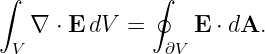
Apply the divergence theorem:
Since
we obtain
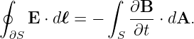
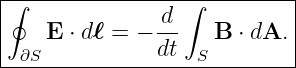
For Faraday’s law, integrate over a fixed surface S:
Apply Stokes’ theorem to the left side:
Because the surface is fixed in space and does not change shape,
Therefore,
For a moving or deforming surface, additional transport terms generally appear; the simple
interchange above is tied to a fixed integration surface.
Solution 6: cylindrical Faraday induction
By symmetry the induced electric field is azimuthal and has constant magnitude around a circular
contour of radius r.
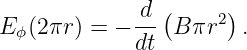
For r < R, Faraday’s law gives
Thus
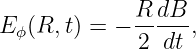
For r > R, only the region of radius R contributes magnetic flux:
so
At r = R, either expression gives
so the idealized solution is continuous.
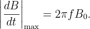
For
we have
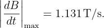
With f = 60 Hz and B0 = 3.0 × 10⁻³ T,
At r = 3.0 cm < R,
| |Eϕ|max | =  (1.131) (1.131) | (88)
|
| = 1.70 × 10⁻² V/m. | (89) |
Thus
At r = 10.0 cm > R,
| |Eϕ|max | =  (1.131) (1.131) | (91)
|
| = 9.05 × 10⁻³ V/m. | (92) |
Therefore,
Inside the changing-flux region the induced field grows linearly with r; outside it falls as 1∕r
because the enclosed changing flux has saturated at πR2B.
Solution 7: cylindrical Ampere–Maxwell induction
With no enclosed conduction current, the integral Ampere–Maxwell law is
By symmetry, B = Bϕϕ.
For r < R,
Hence
For r > R,
so
At r = R, both expressions give
Using
at r = 0.020 m,
| Bϕ | = 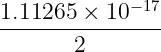 (0.020)(2.0 × 10¹⁰) (0.020)(2.0 × 10¹⁰) | (101)
|
| = 2.23 × 10⁻⁹ T. | (102) |
Thus
At r = 0.100 m,
| Bϕ | = 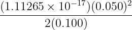 (2.0 × 10¹⁰) (2.0 × 10¹⁰) | (104)
|
| = 2.78 × 10⁻⁹ T. | (105) |
Therefore,
This is the electric-field analogue of Exercise 6: changing electric flux generates circulating
magnetic field.
Solution 8: reconstruct the sources from specified fields
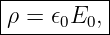
The electric field is
Its divergence is
Gauss’s law therefore gives
The curl of this electric field is zero because it has only an x component and that component
depends only on x and t:
Since B = 0, also
Therefore Faraday’s law is satisfied.
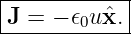
Now use the Ampere–Maxwell equation. Since B = 0,
But
Hence
Finally,
and the reconstructed current is spatially uniform, so
Thus
The sources inferred independently from Maxwell’s equations are automatically compatible with
charge conservation.
Solution 9: why the Ampere–Maxwell integral is surface independent
Reverse the orientation of S2 and join it to S1. The two surfaces form a closed surface
Sc.
The difference between the effective currents is
Apply the divergence theorem:
Evaluate the divergence:
∇⋅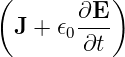 | = ∇⋅ J + 𝜖0 (∇⋅ E) (∇⋅ E) | (120)
|
| = ∇⋅ J + 𝜖0  | (121)
|
| = ∇⋅ J +  . . | (122) |
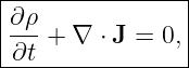
Charge continuity states
Therefore the integrand is zero everywhere, giving
Without the displacement-current term, the divergence would be simply ∇⋅ J = −∂ρ∕∂t, which
need not vanish during charge accumulation. The magnetic circulation around one contour would
then depend on which spanning surface was chosen. Maxwell’s correction removes that
inconsistency.
Solution 10: propagation of Maxwell’s divergence constraints
Take the divergence of Faraday’s law:
The divergence of a curl is identically zero, so
Thus if ∇⋅ B = 0 at the initial time, ideal Maxwell evolution preserves it.
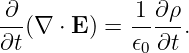
Now take the divergence of the Ampere–Maxwell law:
Divide by μ0𝜖0:
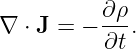
From charge continuity,
Therefore,
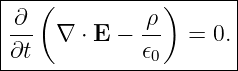
Rearranging,
The implication is important for analytical and numerical field evolution: initial fields must satisfy
the divergence constraints. The ideal continuous equations preserve those constraints thereafter
when the sources satisfy continuity. Numerical discretization can introduce constraint error, so
computational electromagnetics often monitors or actively controls discrete divergence
errors.
Solution 11: plane-wave precursor directly from the curl equations
Let
The electric field has only an x component, so its curl has only a y component:
| (∇× E)y | =  | (133)
|
| = −kE0 sin ϕ. | (134) |
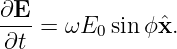
The time derivative of the magnetic field is
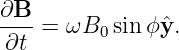
Faraday’s law gives
For nontrivial fields,
Next compute the magnetic curl. Since only By is nonzero,
| (∇× B)x | = − | (138)
|
| = kB0 sin ϕ. | (139) |
Also,
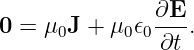
The source-free Ampere–Maxwell equation gives
so
Use the first relation to write
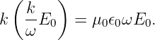
Substitute into the second:
Cancel E0 and multiply by ω:
Therefore,
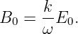
From kE0 = ωB0,
so
The wavelength follows from
For f = 1.57542 × 10⁹ Hz,
| λ | = 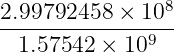 | (150)
|
| ≈ 0.1903 m. | (151) |
Hence,
This result has been obtained directly from Maxwell’s curl equations, before deriving the
second-order wave equation.
Solution 12: reject a longitudinal vacuum-wave candidate
The proposed electric field is
Its divergence is
| ∇⋅ E | =  | (154)
|
| = −kE0 sin(kz − ωt). | (155) |
In source-free vacuum, Gauss’s electric law requires
For nonzero k and nonzero E0, the proposed field does not satisfy that condition for all space and
time. It therefore cannot be a source-free vacuum plane wave.
Because the field has only a z component that depends only on z and t,
With B = 0, Faraday’s law alone is satisfied. This demonstrates why one cannot validate an
electromagnetic field by checking only one of Maxwell’s equations. The entire coupled system must
hold simultaneously.
For a propagating source-free plane wave, Gauss’s electric law rules out a varying electric
component parallel to the propagation direction. This is the beginning of the transversality result
developed more fully in the wave lessons.
Solution 13: recover electrostatics and magnetostatics as limits
Set all time derivatives to zero. Maxwell’s equations become
and
In a simply connected region, ∇× E = 0 permits a scalar potential representation
The magnetic curl equation reduces to the ordinary magnetostatic Ampere law. Both divergence
laws remain unchanged because neither contained an explicit time derivative to begin
with.
Gauss’s magnetic law must remain because magnetostatics still requires magnetic fields to have
zero net flux through every closed surface. The static limit removes time coupling; it does not
remove the geometric constraint on B.
Solution 14: source-free does not mean field-free
For case (a),
is spatially uniform and static. Therefore
With B = 0, all four source-free static Maxwell equations are satisfied. This is a valid local vacuum
solution.
For case (b), a uniform static magnetic field also has
Thus it too is a valid source-free local vacuum solution.
For case (c),
has
Therefore it requires
so it is not source-free.
For case (d), the field from Exercise 4 has
but
Thus it requires
so it is not source-free.
The first two cases make the key point: ρ = 0 and J = 0 do not imply E = 0 and B = 0.
Solution 15: Julia finite-difference check of divergence and curl
For the specified constants, the exact electric-field results are
and
For the magnetic field,
and
One compact Julia implementation is
using LinearAlgebra

alpha, beta, gamma = 2.0, -1.0, 4.0
b = 3.0
h = 1.0e-5
r0 = [0.7, -0.4, 1.1]

E(r) = [alpha*r[1], beta*r[2], gamma*r[3]]
B(r) = [-b*r[2], b*r[1], 0.0]

\href{https://physicslibrary.org/encyclopedia/Bijective.html}{Function} partial(F, r, component, coordinate, h)
rp = copy(r)
rm = copy(r)
rp[coordinate] += h
rm[coordinate] -= h
return (F(rp)[component] - F(rm)[component])/(2h)
end

function divF(F, r, h)
return partial(F,r,1,1,h) +
partial(F,r,2,2,h) +
partial(F,r,3,3,h)
end

function curlF(F, r, h)
cx = partial(F,r,3,2,h) - partial(F,r,2,3,h)
cy = partial(F,r,1,3,h) - partial(F,r,3,1,h)
cz = partial(F,r,2,1,h) - partial(F,r,1,2,h)
return [cx, cy, cz]
end

println("div E = ", divF(E,r0,h))
println("curl E = ", curlF(E,r0,h))
println("div B = ", divF(B,r0,h))
println("curl B = ", curlF(B,r0,h))
The numerical output should be close to
div E = 5.0
curl E = [0.0, 0.0, 0.0]
div B = 0.0
curl B = [0.0, 0.0, 6.0]
up to floating-point and finite-difference roundoff. The exercise connects the geometric definitions
of divergence and curl with the discrete derivative operations used in computational field
solvers.
1 What EM15E1 adds to the series
EM15 assembled Maxwell’s four equations into a coherent field theory. EM15E1 pushes that
synthesis further by requiring the equations to be used together.
The most important structural results are:
and, for the transverse plane-wave trial fields,
The next natural step is to take the curl of the curl equations and derive the second-order
electromagnetic wave equations for E and B directly.
References
[1] David J. Griffiths, Introduction to Electrodynamics, 4th ed., Cambridge University
Press, 2017.
[2] Edward M. Purcell and David J. Morin, Electricity and Magnetism, 3rd ed.,
Cambridge University Press, 2013.
[3] Samuel J. Ling, Jeff Sanny, and William Moebs, University Physics, Volume 2,
OpenStax, 2016, sections on Maxwell’s equations and electromagnetic waves.
[4] Richard P. Feynman, Robert B. Leighton, and Matthew Sands, The Feynman Lectures
on Physics, Volume II, Addison-Wesley, 1964, chapters on Maxwell’s equations and
electromagnetic radiation.
[5] Massachusetts Institute of Technology, 8.02 Physics II: Electricity and Magnetism,
MIT OpenCourseWare, materials on Maxwell’s equations, Gauss’s law, Faraday
induction, the Ampere–Maxwell law, and electromagnetic waves.

![[parent]](https://images.physicslibrary.org/images/uparrow.png)
![[ ]
ρ-
[∇ ⋅ E ] = 𝜖0 ,](https://images.physicslibrary.org/cache/objects/1238/make4ht/ElectromagneticWavesMaxwellsEquationsAsACompleteSystemExercisesAndCompleteWorkedSolutions4x.png)
![[ ]
∂B
[∇ × E ] = ---- ,
∂t](https://images.physicslibrary.org/cache/objects/1238/make4ht/ElectromagneticWavesMaxwellsEquationsAsACompleteSystemExercisesAndCompleteWorkedSolutions5x.png)
![[ ]
∂E-
[∇ × B ] = [μ0J ] = μ0𝜖0∂t .](https://images.physicslibrary.org/cache/objects/1238/make4ht/ElectromagneticWavesMaxwellsEquationsAsACompleteSystemExercisesAndCompleteWorkedSolutions6x.png)
![3 2
[E] = V/m, [B] = T, [ρ] = C/m , [J ] = A/m .](https://images.physicslibrary.org/cache/objects/1238/make4ht/ElectromagneticWavesMaxwellsEquationsAsACompleteSystemExercisesAndCompleteWorkedSolutions7x.png)



















![V/m
[∇ ⋅ E ] =---- = V/m2.
m](https://images.physicslibrary.org/cache/objects/1238/make4ht/ElectromagneticWavesMaxwellsEquationsAsACompleteSystemExercisesAndCompleteWorkedSolutions40x.png)
![--C--
[𝜖0] = V m ,](https://images.physicslibrary.org/cache/objects/1238/make4ht/ElectromagneticWavesMaxwellsEquationsAsACompleteSystemExercisesAndCompleteWorkedSolutions41x.png)
![[∇ × E] = V/m2.](https://images.physicslibrary.org/cache/objects/1238/make4ht/ElectromagneticWavesMaxwellsEquationsAsACompleteSystemExercisesAndCompleteWorkedSolutions44x.png)

![[ ]
∂B-- = T-= V/m2.
∂t s](https://images.physicslibrary.org/cache/objects/1238/make4ht/ElectromagneticWavesMaxwellsEquationsAsACompleteSystemExercisesAndCompleteWorkedSolutions46x.png)
![[∇ × B ] = T/m.](https://images.physicslibrary.org/cache/objects/1238/make4ht/ElectromagneticWavesMaxwellsEquationsAsACompleteSystemExercisesAndCompleteWorkedSolutions47x.png)
![[μ0] = T m/A,](https://images.physicslibrary.org/cache/objects/1238/make4ht/ElectromagneticWavesMaxwellsEquationsAsACompleteSystemExercisesAndCompleteWorkedSolutions48x.png)
![T-m--A-
[μ0J ] = A m2 = T/m.](https://images.physicslibrary.org/cache/objects/1238/make4ht/ElectromagneticWavesMaxwellsEquationsAsACompleteSystemExercisesAndCompleteWorkedSolutions49x.png)
![[μ 𝜖 ] = s2∕m2,
0 0](https://images.physicslibrary.org/cache/objects/1238/make4ht/ElectromagneticWavesMaxwellsEquationsAsACompleteSystemExercisesAndCompleteWorkedSolutions50x.png)