Electromagnetic Waves, Antennas, and RF: Electric Flux
EM05 introduced the Electric Field E(r) as a vector field in space. EM06 asks a new question: how
much of that field passes through a surface?
The answer is described by electric flux. Flux combines two pieces of geometry:
- the strength and direction of the electric field, and
- the size and orientation of the surface.
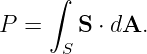
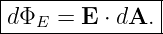
The central mathematical operation is the dot product. For a small oriented surface element
dA,
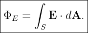
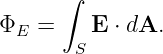
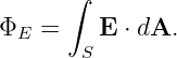
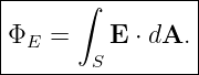
For a finite surface,
This geometric language prepares the way for Gauss’s Law. EM06 develops flux itself first so that
the later law can be understood as physics rather than as an unfamiliar integral formula
[1, 2, 3, 5].
1 Why a surface needs an orientation
A scalar area tells us only how large a surface is. Flux also depends on which way the surface
faces.
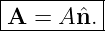
For a flat surface of area A, choose a unit normal vector n perpendicular to the surface. The
corresponding area vector is
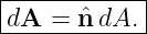
For an infinitesimal surface patch,
The direction of the area vector is not tangent to the surface. It is perpendicular to the
surface.
For an open surface, either of the two opposite normals may be chosen. Reversing the chosen
normal reverses the sign of the flux.
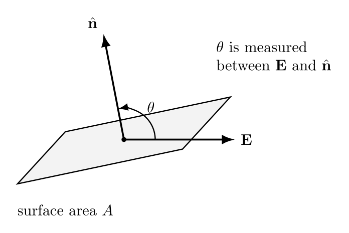
Figure. A flat surface is assigned a normal direction n. The angle 𝜃 used in electric flux is
the angle between E and the surface normal, not the angle between E and the surface itself.
2 Flux through a uniform flat surface
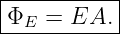
Suppose the electric field is uniform over a flat surface. Then the flux is
Using the dot-product definition,
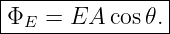
where 𝜃 is the angle between E and the chosen surface normal. Therefore,
This formula is the simplest electric-flux relation.
2.1 Maximum positive flux
If the field points in the same direction as the surface normal,
so
The field passes through the surface as directly as possible.
2.2 Zero flux
If the field lies parallel to the surface, then it is perpendicular to the normal:
Therefore,
A strong electric field can therefore produce zero flux through a particular surface if the field runs
along that surface rather than through it.
2.3 Negative flux
If the field points mostly opposite the chosen normal,
then
and the flux is negative.
The sign is therefore an orientation statement, not a statement that the electric-field magnitude is
negative.
3 Projected area interpretation
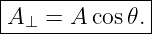
The factor
has a simple geometric interpretation. It is the area of the surface projected onto a plane
perpendicular to the electric field.
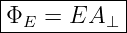
Thus
with
A tilted surface presents a smaller effective area to the field.
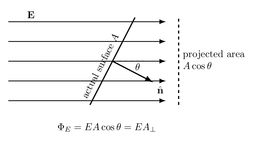
Figure. A tilted surface of actual area A presents the projected area A cos 𝜃 to a uniform
field. This provides a geometric interpretation of the dot product in ΦE = EA cos 𝜃.
4 Units of electric flux
From
we have
and
Therefore,
Electric flux is not measured in coulombs. It is a field-times-area quantity.
5 From one flat patch to a general surface
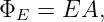
The simple formula
Works only when the field is effectively uniform over the surface and the surface has one
well-defined normal direction.
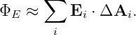
For a curved surface, or for a field that changes from point to point, divide the surface into many
small patches.
For patch i,
Adding all patches gives
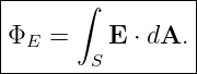
In the limit of infinitesimal patches,
This is a surface integral.
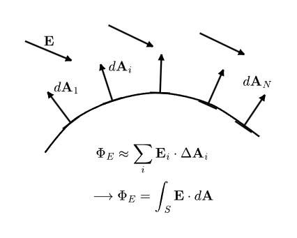
Figure. A curved surface is approximated by many small patches. Each patch has its own
local normal and area vector dA. The total flux is the sum, in the continuum limit, of
E ⋅ dA over the surface.
6 What the dot product does locally
At every small patch,
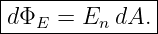
Only the component of E normal to the surface contributes. Define
Then
The tangential component of the electric field does not contribute to flux through that
patch.
7 Open surfaces and closed surfaces
An open surface has an edge. Examples include a disk, a rectangle, or a hemisphere without its flat
base. Its normal orientation must be specified.
A closed surface completely encloses a volume. Examples include a sphere, a cube, or a sealed
irregular surface.
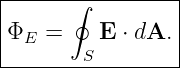
For a closed surface, the standard convention is
The total flux through a closed surface is written
With the outward-normal convention:
- field leaving the enclosed volume contributes positive flux;
- field entering the enclosed volume contributes negative flux.
8 A uniform field through a closed box
Consider a constant electric field E = E0x and a rectangular box.
The right face has outward normal +x, so its flux is positive. The left face has outward normal −x,
so its flux is negative with equal magnitude. The other faces have normals perpendicular to E, so
their flux is zero.
Hence the total closed-surface flux is
This does not mean the electric field is zero. It means as much field passes into the box as passes
out.
9 Field lines are a picture, not the definition
Electric-field lines are often used to visualize flux. A surface crossed by many field lines is drawn as
having large flux, while a surface nearly parallel to the lines is drawn as having small
flux.
This picture is useful, but flux is not literally a count of physical lines. Field lines are a
visualization convention. The mathematical definition is
The field itself is continuous even though a diagram contains only a finite number of drawn
lines.
10 Flux of a point-charge field through a centered sphere
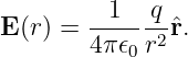
EM05 showed that a point charge q at the origin produces
Now surround the charge by a sphere of radius r centered on the charge.
At every point on the sphere, the outward area vector is radial:
Therefore,
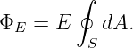
The field magnitude is the same everywhere on the sphere, so
The area of the sphere is
Thus
| ΦE | = 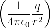 (4πr2) (4πr2) | (37)
|
| =  . . | (38) |
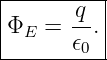
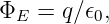
Therefore,
The radius cancels. A larger sphere has weaker field magnitude, but it also has proportionally
larger area.
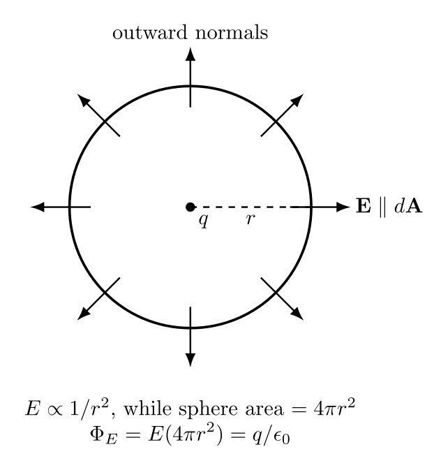
Figure. For a sphere centered on a point charge, the electric field and outward area vector
are parallel everywhere. The 1∕r2 decrease of field magnitude is exactly balanced by the
4πr2 growth of spherical area.
This result is a preview of Gauss’s law. At this stage it has been derived only for a sphere centered
on a point charge, using the known Coulomb field. EM07 will state and analyze the much more
general law for arbitrary closed surfaces.
11 Worked examples
Example 1: uniform field normal to a surface
A uniform electric field has magnitude
It passes normally through a flat surface of area
With 𝜃 = 0,
| ΦE | = EA cos 0 | (42)
|
| = (200)(0.50) | (43)
|
| = 100 N m2∕C. | (44) |
Hence
Example 2: tilted flat surface
Let
where 𝜃 is measured from E to the surface normal.
Then
| ΦE | = EA cos 𝜃 | (47)
|
| = (300)(0.20) cos 60∘ | (48)
|
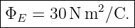
| = 30 N m2∕C. | (49) |
Thus
Example 3: field parallel to the surface
If a field of any magnitude lies exactly parallel to a flat surface, then the angle to the normal is
90∘. Therefore,
A nonzero field can therefore have zero flux through a particular surface.
Example 4: reversing the surface orientation
Suppose a flat surface has flux
for the chosen normal n.
If the surface orientation is reversed,
then
Hence
The physical field has not changed. Only the orientation convention changed.
Example 5: a nonuniform field through a plane
Let
and consider a rectangular surface lying in the plane x = a, with outward normal +x and area
A.
Every point on that surface has the same coordinate x = a, so
Thus
| ΦE | = ∫
SE ⋅ dA | (58)
|
| = ∫
SαadA | (59)
|
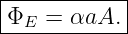
| = αaA. | (60) |
Therefore,
The field is nonuniform in space generally, but it is uniform over this particular constant-x
surface.
Example 6: net flux through a box in a uniform field
Take
Let the two faces normal to the x axis each have area A.
The right face contributes
The left face contributes
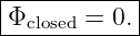
The other four faces contribute zero. Thus
Example 7: centered point charge and spherical surface
Let
For a centered sphere, the flux found above is
Using
we obtain approximately
The answer does not depend on the radius of the centered sphere.
12 Common mistakes
12.1 Using the angle to the surface instead of the normal
In
𝜃 is the angle between E and n.
If a problem gives the angle between the field and the surface itself, convert it to the
complementary angle before using the cosine form.
12.2 Treating area as a scalar when orientation matters
The flux integrand uses
not merely dA.
12.3 Assuming zero flux means zero field
A field parallel to a surface produces zero flux through that surface even though the field can be
large.
12.4 Assuming flux is always positive
Flux can be positive, negative, or zero depending on the chosen orientation and local field
direction.
12.5 Counting drawn field lines literally
Field-line diagrams illustrate direction and relative density. Flux is defined by an integral, not by
counting artistic lines in a sketch.
12.6 Applying EA cos 𝜃 to any surface without checking assumptions
The simple formula requires a uniform field over a flat surface, or at least conditions under which
the field and normal are effectively constant. The general formula is
13 Why electric flux matters later
Electric flux is much more than a geometric exercise. The same mathematical structure appears
repeatedly in Electromagnetism.
Gauss’s law will relate closed-surface electric flux to enclosed charge:
Later, magnetic flux will use the analogous quantity
and Faraday’s law will relate changing magnetic flux to circulation of the electric field.
Still later, electromagnetic power flow through a surface will use the Poynting vector:
Thus the same geometric idea developed here becomes essential for fields, induction, waves,
antennas, apertures, and RF power flow.
Summary
The essential results of EM06 are:
The next lesson, EM07, introduces Gauss’s law and explains when symmetry allows electric fields
to be obtained from closed-surface flux with remarkable efficiency.
References
[1] David J. Griffiths, Introduction to Electrodynamics, 4th ed., Cambridge University
Press, 2017.
[2] Samuel J. Ling, Jeff Sanny, and William Moebs, University Physics, Volume 2,
OpenStax, 2016, sections on electric flux and Gauss’s law.
[3] Edward M. Purcell and David J. Morin, Electricity and Magnetism, 3rd ed.,
Cambridge University Press, 2013.
[4] Richard P. Feynman, Robert B. Leighton, and Matthew Sands, The Feynman Lectures
on Physics, Volume II, Addison-Wesley, 1964, chapters on electrostatics and Gauss’s law.
[5] Massachusetts Institute of Technology, 8.02 Physics II: Electricity and Magnetism,
MIT OpenCourseWare, materials on electric flux and Gauss’s law.









![[E ] = N/C](https://images.physicslibrary.org/cache/objects/1219/make4ht/ElectromagneticWavesElectricFlux17x.png)
![[A] = m2.](https://images.physicslibrary.org/cache/objects/1219/make4ht/ElectromagneticWavesElectricFlux18x.png)
![|----------------|
|[ΦE ] = N m2 ∕C.|
-----------------](https://images.physicslibrary.org/cache/objects/1219/make4ht/ElectromagneticWavesElectricFlux19x.png)