Electromagnetic Waves, Antennas, and RF: Ampère’s Law and Symmetry
EM11 used the Biot–Savart law to add magnetic-field contributions from many current elements.
That source-integral method is systematic, but it can become mathematically expensive even when
the current distribution has a simple symmetry.
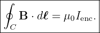
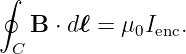
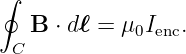
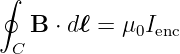
Ampère’s law provides a second magnetostatic tool. Instead of summing contributions from every
source element, it relates the circulation of the magnetic field around a closed path directly to the
current enclosed by that path:
The central lesson of this article parallels EM07 on Gauss’s Law:
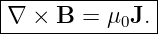
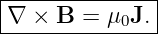
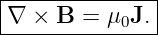
For steady currents, Ampère’s law is fully equivalent to the magnetostatic curl equation
The time-varying case will later require Maxwell’s additional displacement-current term
[1, 2, 3, 5].
1 Magnetic circulation
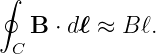
The integral
is a line integral around a closed curve C.
For a small path element,
where 𝜃 is the angle between the local magnetic field and the local direction of the
path.
Three cases are immediately useful:
- if B is tangent to the path in the same direction, then B ⋅ dℓ = B dℓ;
- if B is perpendicular to the path, then the contribution is zero;
- if B is constant along a path segment, it may be taken outside the integral over that
segment.
These geometric simplifications are what make a carefully chosen Amperian path powerful.
2 Orientation and enclosed current
The direction in which the closed path is traversed determines the positive normal of any surface
bounded by the path. Use the right-hand rule:
- curl the fingers of the right hand in the positive traversal direction around C;
- the thumb gives the positive surface-normal direction;
- currents piercing the surface in the thumb direction count as positive enclosed current.
Thus Ienc is an oriented quantity, not merely the sum of current magnitudes.
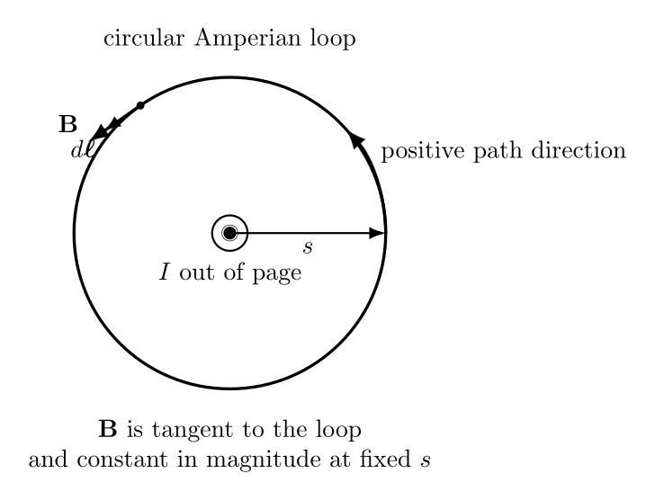
Figure. A circular Amperian loop around a long straight wire. The magnetic field is
tangent to the circle and has constant magnitude at fixed radius.
3 Why symmetry matters
Ampère’s law always relates the closed-path circulation to enclosed steady current, but it does
not automatically provide the local field magnitude.
To solve directly for B, one usually seeks a path for which symmetry guarantees one or more of the
following:
- the direction of B is known;
- B is tangent to the path where it contributes;
- B has the same magnitude along a contributing path segment;
- other path segments make zero contribution because B ⊥ dℓ.
This is the magnetic counterpart of selecting a Gaussian surface that matches an electric-field
symmetry.
4 Example 1: a known circular field
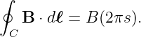
Suppose a magnetic field has constant magnitude
and is everywhere tangent to a circular path of radius
Then
| ∮
CB ⋅ dℓ | = B ∮
Cdℓ | (8)
|
| = B(2πs). | (9) |
Therefore,
| ∮
CB ⋅ dℓ | = (2.0 × 10⁻⁴)2π(5.0 × 10⁻²) | (10)
|
| = 6.28 × 10⁻⁵ T m. | (11) |
The line integral measures magnetic circulation around the path.
5 The infinitely long straight wire
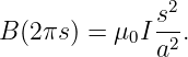
For an infinitely long straight wire carrying current I, cylindrical symmetry implies that
magnetic-field lines are circles centered on the wire. At fixed distance s from the wire, the
magnitude B is constant.
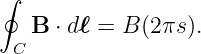
Choose a circular Amperian loop of radius s. Then
The enclosed current is simply I, so Ampère’s law gives
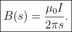
Hence,
This is exactly the result derived by direct Biot–Savart integration in EM11, but symmetry makes
the Ampère-law derivation much shorter.
6 Example 2: field around a straight wire
Let
Then
| B | = 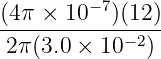 | (16)
|
| = 8.0 × 10⁻⁵ T. | (17) |
Thus,
7 A cylindrical wire with uniform current density
Now suppose the wire has radius a and carries total current I distributed uniformly across its cross
section.
The uniform current density is
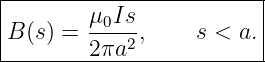
For an Amperian circle of radius s < a, only the current inside radius s is enclosed:
| Ienc | = Jπs2 | (20)
|
| = I . . | (21) |
Ampère’s law gives
Therefore, inside the wire,
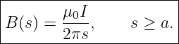
Outside the wire, s ≥ a, the entire current is enclosed, so
Thus the field increases linearly with radius inside a uniformly current-filled wire and decreases as
1∕s outside.
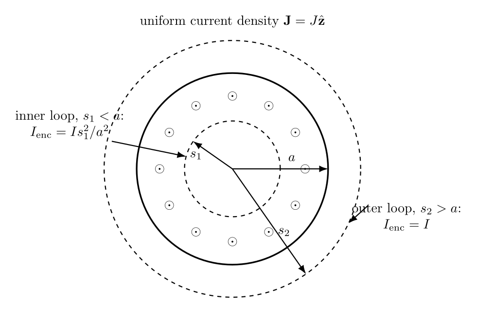
Figure. A uniformly current-filled cylindrical wire. An inner Amperian loop encloses only
the fraction of current lying inside its radius.
8 Example 3: field inside a uniform-current wire
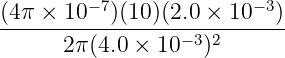
A cylindrical wire has
Find the field at
Because s < a,
| B | =  | (27)
|
| =  | (28)
|
| = 2.5 × 10⁻⁴ T. | (29) |
So
9 The ideal long solenoid
A solenoid is a helical winding with many turns per unit length. Let
be the number of turns per unit length.
For a sufficiently long ideal solenoid, symmetry and the long-solenoid approximation
imply:
- the magnetic field inside is approximately uniform and parallel to the solenoid axis;
- the external field is small compared with the interior field away from the ends.
Choose a rectangular Amperian path with one long side of length ℓ inside the solenoid and parallel
to the field, and the opposite long side outside where the idealized field is approximately zero. The
short sides are perpendicular to B and contribute zero.
Therefore,
The number of windings piercing the surface is
so the enclosed current is
Ampère’s law gives
Hence,
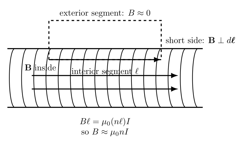
Figure. A rectangular Amperian path for an ideal long solenoid. The interior segment is
parallel to the nearly uniform magnetic field; the exterior contribution is idealized as
negligible.
10 Example 4: ideal-solenoid field
Let
Then
| B | = μ0nI | (38)
|
| = (4π × 10−7)(1200)(0.80) | (39)
|
| = 1.21 × 10⁻³ T. | (40) |
Therefore,
11 The ideal toroid
A toroid may be viewed as a solenoid bent into a closed ring. Suppose it has N turns carrying
current I.
For an ideal toroid, symmetry implies that the magnetic field inside the winding region is
approximately azimuthal and depends only on the distance s from the toroid’s central
axis.
Choose a circular Amperian loop of radius s lying within the winding region. The field is tangent
to the loop and has constant magnitude there, so
The loop encloses N current crossings, so
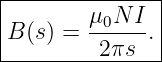
Thus,
or
For the idealized toroid, the field is approximately zero in the central hole and outside the winding
region because an appropriate Amperian loop there encloses zero net current.
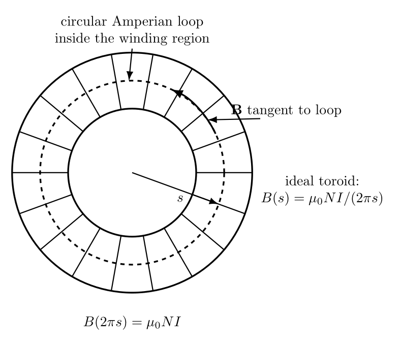
Figure. Circular Amperian path through an ideal toroid. Inside the winding region, B is
tangent to the path and has constant magnitude at fixed radius.
12 Example 5: ideal-toroid field
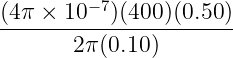
Let
Then
| B | =  | (47)
|
| =  | (48)
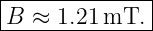
|
| = 4.0 × 10⁻⁴ T. | (49) |
So
13 When Ampère’s law is true but not directly useful
Consider two separated current-carrying wires or a finite bent Conductor with little
symmetry. Ampère’s law still gives the circulation around any chosen closed path, but
the local field magnitude may vary around the path and may not remain tangent to
it.
Then one cannot replace
with a simple product such as
The difficulty is not a failure of Ampère’s law. The difficulty is that symmetry is insufficient to
remove B from the line integral.
In such cases, Biot–Savart integration, superposition, numerical field methods, or later
Maxwell-equation techniques may be more useful.
14 Example 6: deciding whether a circular path is useful
Suppose a current distribution contains a single infinitely long straight wire, but the proposed
circular path is not centered on the wire.
Ampère’s law still gives
However, the distance from the wire to points on the off-center circle changes around the path.
Therefore B is not constant on the path, and the field is not everywhere tangent to that
circle.
So the off-center circle is a poor path for directly solving for B.
The correct symmetry-matched path is a circle centered on the wire.
15 From integral Ampère’s law to the differential form
Stokes’ theorem relates the circulation of a vector field around a closed curve to the flux of its curl
through any surface bounded by that curve:
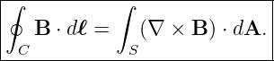
Ampère’s law states
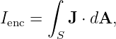
Using the current-density relation
we obtain
Therefore,
For arbitrary surfaces in magnetostatics, the local relation is
This equation connects directly back to the curl operator introduced in EM03.
16 Example 7: verify the differential form
Consider the field
The curl has only a z component:
| (∇× B)z | =  − − | (61)
|
| =  − − | (62)
|
| = μ0J0. | (63) |
Thus,
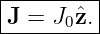
This corresponds to the current density
17 The magnetostatic limitation
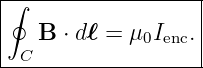
The form
is the magnetostatic form of Ampère’s law. It assumes steady-current conditions.
For genuinely time-varying electromagnetic fields, this expression is incomplete. Maxwell
discovered that a changing electric flux contributes to magnetic-field circulation even where no
conduction current passes through the chosen surface.
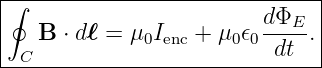
The corrected law, introduced later in this series, has the structure
For EM12, the important point is only the boundary of validity:
The displacement-current term will become essential when the series turns to electromagnetic
waves and antennas.
18 Common mistakes
- Mistake: assuming Ampère’s law gives B directly for every current geometry. The law
gives circulation; symmetry is what may turn the line integral into a simple algebraic
expression.
- Mistake: using total current when an Amperian loop encloses only part of a distributed
current.
- Mistake: forgetting the orientation sign of enclosed current.
- Mistake: assuming a circular Amperian path is useful merely because it is a circle. It
must be centered on the symmetry axis for the straight-wire problem.
- Mistake: treating the ideal solenoid and toroid formulas as exact for every finite
winding geometry.
- Mistake: applying the magnetostatic Ampère law without modification to
time-varying antenna currents.
19 What EM12 adds to the series
EM11 introduced the magnetostatic source integral
EM12 adds a complementary circulation law:
With sufficient symmetry, that law gives the straight-wire, solenoid, and toroid fields with very
little integration.
Using Stokes’ theorem, the same magnetostatic physics can be written locally as
The next stage of the series will move from magnetostatics toward time-varying fields and
induction, where electric and magnetic fields begin to generate one another dynamically.
References
[1] David J. Griffiths, Introduction to Electrodynamics, 4th ed., Cambridge University
Press, 2017.
[2] Edward M. Purcell and David J. Morin, Electricity and Magnetism, 3rd ed.,
Cambridge University Press, 2013.
[3] Samuel J. Ling, Jeff Sanny, and William Moebs, University Physics, Volume 2,
OpenStax, 2016, sections on Ampère’s law, solenoids, and toroids.
[4] Richard P. Feynman, Robert B. Leighton, and Matthew Sands, The Feynman Lectures
on Physics, Volume II, Addison-Wesley, 1964, chapters on magnetic fields, circulation,
and Maxwell’s equations.
[5] Massachusetts Institute of Technology, 8.02 Physics II: Electricity and Magnetism,
MIT OpenCourseWare, materials on Ampère’s law, solenoids, toroids, and
magnetic-field symmetry.