1 Definition
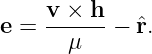
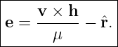
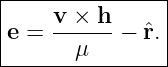
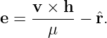
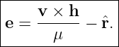
In ideal Newtonian two-body motion, the eccentricity vector is the conserved, dimensionless
vector
where
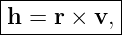
Here r is the position of the orbiting body relative to the central body, v = dr∕dt is its relative
velocity, h is the specific angular-momentum vector, and μ = G(M + m) ≈ GM is the
gravitational parameter.
The eccentricity vector has two defining geometric properties:
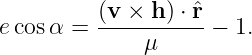
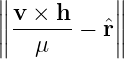
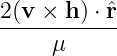
and, for e > 0,
Thus one vector contains both the shape and an important part of the orientation of a Keplerian
orbit. Its magnitude e is the ordinary scalar eccentricity of the conic, while its direction fixes the
periapsis line within the orbital plane.
The vector is also the dimensionless form of the Laplace–Runge–Lenz vector. If
then
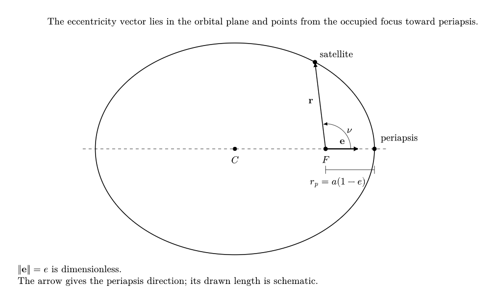
Figure 1. The eccentricity vector lies in the orbital plane and points from the occupied focus
toward periapsis. Its magnitude is the dimensionless eccentricity e, not a physical distance.
A useful distinction is
where rp is the physical focus-to-periapsis distance and c is the center-to-focus distance of an
ellipse. These three quantities should not be confused: only e is the magnitude of the eccentricity
vector.
For a circular orbit,
A circle has no unique periapsis, so the zero vector correctly carries no preferred in-plane
direction.
2 Why introduce the eccentricity vector?
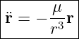
The governing equation for ideal two-body motion is
One conserved vector follows immediately:
Because the gravitational acceleration is parallel to r,
Thus h is constant.
The angular-momentum vector tells us the orbital plane and its positive normal direction, but it
does not identify where periapsis lies inside that plane. Rotating an ellipse about its focus without
changing its plane leaves h unchanged. A second conserved vector is therefore useful: one that
lies in the orbital plane and singles out the periapsis direction. Equation (1) is that
vector.
The remaining question is not what the eccentricity vector is, but why Newton’s inverse-square law
produces exactly this combination. The following derivation answers that question.
3 Derivation: searching for an in-plane conserved vector
The formula in Eq. (1) looks arbitrary if it is simply quoted. A more instructive route is to search
for a second conserved quantity.
The angular-momentum vector h is perpendicular to the orbital plane, while v lies in that plane.
Therefore
is itself in the orbital plane. This makes it a natural candidate from which to construct a vector
that could identify a preferred in-plane direction.
The key question is:
What is the time derivative of v × h under an inverse-square central force?
If that derivative matches the derivative of another simple in-plane vector, their difference will be
conserved. That is exactly what happens.
4 A needed kinematic identity: radial distance and radial direction
Before differentiating v × h, we need two facts about the position vector. Write
Differentiating gives
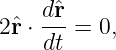
Because r has unit magnitude,
Differentiating this identity gives
so
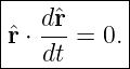
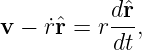
Thus the derivative of a unit vector is perpendicular to the unit vector itself:  changes direction,
not magnitude.
changes direction,
not magnitude.
Dot Eq. (14) with r:
| r ⋅ v | = ṙ (r ⋅r) + r(r ⋅ ) ) | (18)
|
| = ṙ. | (19) |
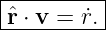
Therefore
This says that the scalar radial rate is simply the component of velocity along the radial unit
vector.
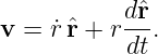
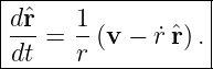
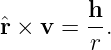
Solving Eq. (14) for the unit-vector derivative,
Only the transverse part of velocity rotates r.
5 The key cross-product identity
Now evaluate
Using h = r × v,
Apply the vector triple-product identity
Then
| r × h | = r(r ⋅ v) − v(r ⋅ r) | (25)
|
| = (rr)ṙ − rv | (26)
|
| = −r . . | (27) |
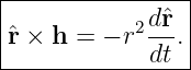
Using Eq. (21),
so
This identity is the algebraic hinge of the eccentricity-vector derivation.
6 Deriving the conserved vector from Newton’s law
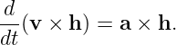
Differentiate v × h:
 (v × h) (v × h) | = 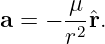 × h + v × × h + v × . . | (30) |
Because  = 0,
= 0,
Newton’s inverse-square acceleration is
Therefore
| a × h | = −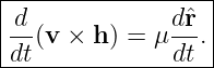 (r × h). (r × h). | (33) |
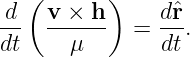
Substitute Eq. (29):
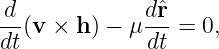
Thus
Now the construction is no longer mysterious. Move the right-hand derivative to the
left:
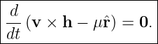
or
Therefore the quantity in parentheses is a conserved vector.
Divide by the constant μ. The conserved dimensionless vector is therefore
This is the eccentricity vector.
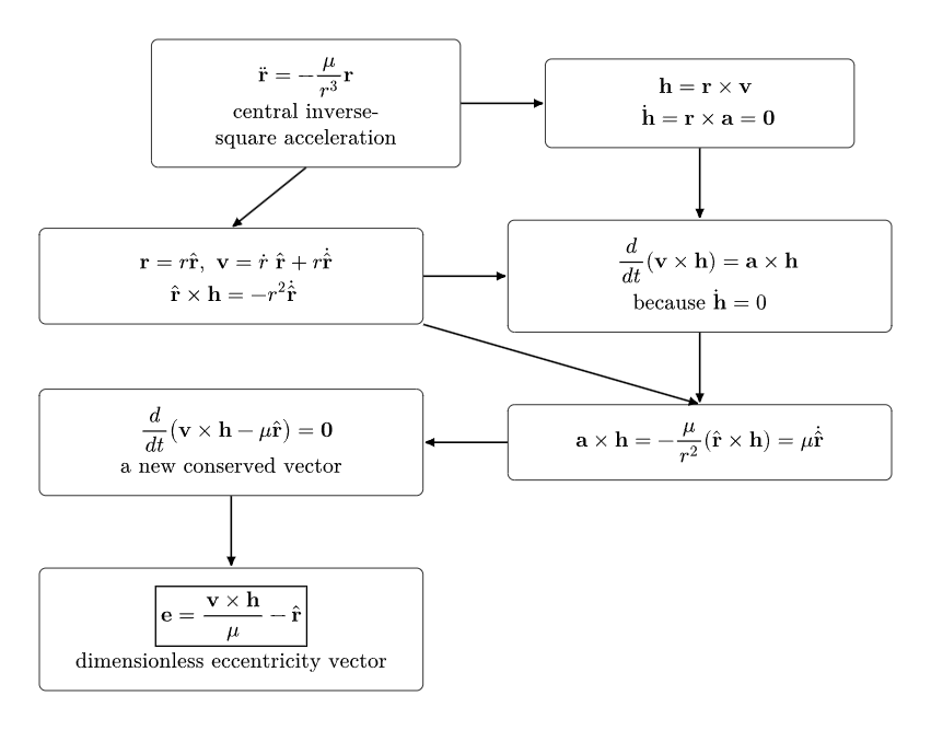
Figure 2. The eccentricity vector emerges because Newton’s inverse-square law makes the
derivatives of v × h and μr identical. Their difference is therefore conserved.
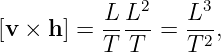
The dimensional check is also revealing. Since
and
the ratio (v × h)∕μ is dimensionless, just like r. Therefore e is dimensionless.
7 Why does this vector point toward periapsis?
Conservation alone does not yet prove that e points toward periapsis. That fact comes from
projecting Eq. (39) onto the radial direction.
Let α be the instantaneous angle between e and r. Then
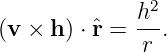
Dot Eq. (39) with r:
Use the scalar triple-product identity,
But
so
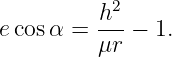
Therefore
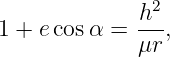
Equation (43) becomes
Rearrange:
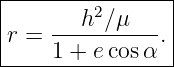
and solve for r:
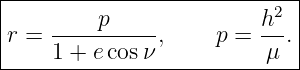
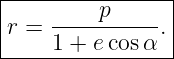
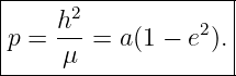
The standard polar equation of a conic with a focus at the origin is written
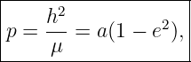
where p is the semilatus rectum. Comparing this geometric conic form with Eq. (50)
identifies
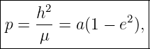
Thus p = h2∕μ is not an arbitrary orbital-mechanics definition; it is the dynamical value of the
conic’s geometrically defined semilatus rectum. Therefore
This is the polar equation of a conic with the central body at the focus.
For e > 0, r is smallest when the denominator is largest, which occurs at
Thus the direction α = 0, namely the direction of e, is the direction of closest approach. That is
periapsis.
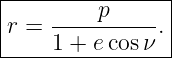
Therefore
Once that fact is established, the angle α is conventionally called the true anomaly ν, so Eq. (53)
becomes
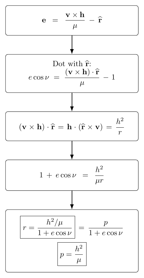
Figure 3. Dotting the eccentricity vector with the radial unit vector produces the conic equation
and identifies p = h2∕μ as the semilatus rectum.
This is one of the most useful results in celestial mechanics: the same vector derived from Newton’s
differential equation simultaneously encodes the orbit’s shape and its orientation within the orbital
plane.
8 Why is its magnitude the conic eccentricity?
The symbol e in Eq. (56) is exactly the geometric eccentricity parameter of the conic. Since that
equation was obtained using
the magnitude of the eccentricity vector is the scalar conic eccentricity.
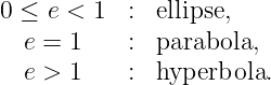
Its value classifies the Kepler orbit:
A circle is the special elliptical case e = 0.
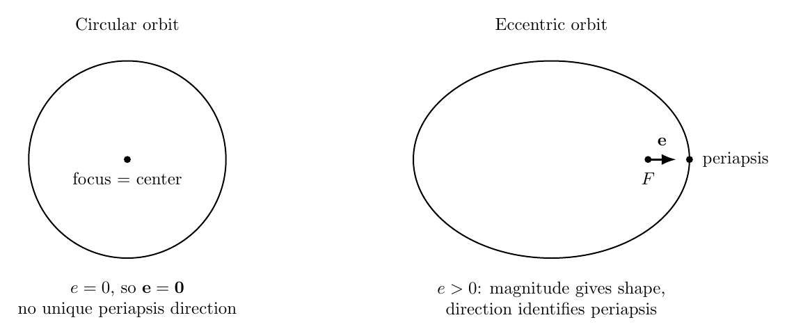
Figure 4. For a circular orbit the eccentricity vector vanishes, so no periapsis direction exists. For
an eccentric orbit its direction selects periapsis and its magnitude measures the conic eccentricity.
This circular limit explains an important singularity in classical orbital elements. If
then the argument of periapsis ω cannot be defined uniquely because there is no distinguished
periapsis direction.
9 Connection with orbital energy
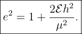
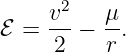
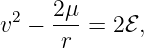
The eccentricity magnitude can also be related directly to the specific mechanical energy
square Eq. (39):
| e2 | = 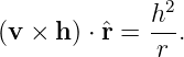 2 2 | (61)
|
| = 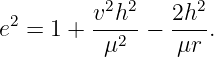 + 1 − + 1 −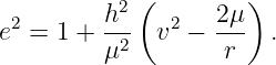 . . | (62) |
Because v lies in the orbital plane while h is normal to it,
so
We already found
Hence
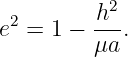
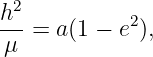
Factor h2∕μ2:
Using Eq. (60),
so
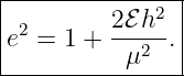
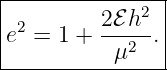
This formula connects the two principal invariants of Kepler motion: angular momentum controls
the orbital plane and transverse scale, while energy controls whether the conic is bound or
unbound. Their combination determines eccentricity.
For an ellipse,
Substituting into Eq. (69),
Therefore
and with Eq. (52),
Thus the semilatus rectum is where Newtonian dynamics, conic geometry, and classical orbital
elements meet.
10 An equivalent Cartesian formula
Equation (39) is compact, but software often uses an equivalent expression containing only r, v,
and scalar dot products. Start with
Apply the triple-product identity:
Hence
Since
Eq. (39) becomes
Both forms are mathematically identical:
The cross-product form is often better for geometric understanding; the expanded form makes the
dependence on radial velocity r ⋅ v = rṙ explicit.
11 A physical reading of the two terms
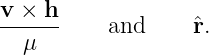
The eccentricity vector can be read as a competition between
The radial unit vector always has magnitude one and continually rotates as the body moves around
the focus. The first term also changes as the velocity direction changes. For an inverse-square force,
Eq. (36) says these two changes are exactly synchronized:
Their difference is therefore frozen in inertial space.
That is the deepest intuition behind Eq. (39): it is not a lucky algebraic combination. It is a
cancellation created by the special 1∕r2 central force.
If the force law is perturbed, for example by Earth’s oblateness, third-body gravity, or atmospheric
drag, the osculating eccentricity vector generally changes slowly with time. Its changing direction
describes apsidal precession, and its changing magnitude describes changes in orbital
shape.
12 The Laplace–Runge–Lenz vector
A closely related conserved quantity is
This is commonly called the Laplace–Runge–Lenz vector, or simply the Runge–Lenz vector in
many mechanics texts. Comparing Eqs. (39) and (82),
The two vectors therefore have exactly the same direction. The normalized form e is particularly
convenient in astrodynamics because its magnitude is immediately the dimensionless orbital
eccentricity.
13 Worked GPS-like numerical example
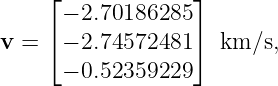
Consider the Earth-centered inertial state
with
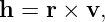
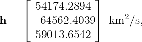
First compute the specific angular momentum,
which gives approximately
with
The position magnitude is
so
Now evaluate
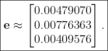
The result is
Its magnitude is
The orbit is therefore a low-eccentricity ellipse.
The specific mechanical energy is
which corresponds to
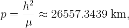
The semilatus rectum obtained dynamically is
while the orbital-element expression gives
The agreement provides a useful implementation check.
The angle between e and r is
which recovers the true anomaly used to generate the state.
Finally, the radial speed is
The positive sign indicates that the spacecraft is moving outward, away from periapsis toward
apoapsis.
14 Implementation recipe from a Cartesian state
Given r, v, and μ, the eccentricity-vector calculation is short:
| r | = ∥r∥, | (101)
|
| h | = r × v, | (102)
|
| e | =  − −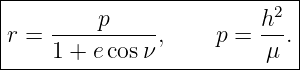 , , | (103)
|
| e | = ∥e∥. | (104) |
For e > 0, the unit periapsis direction is
This is exactly the P axis of the perifocal PQW frame.
In numerical software, one should treat very small e carefully. As e → 0, the magnitude of e
becomes small and its normalized direction becomes sensitive to numerical noise because a circular
orbit has no physically unique periapsis.
15 What to remember
The eccentricity vector can be understood through a compact chain of ideas:
Its final form is
Its magnitude is
its direction is toward periapsis, and its projection onto r immediately generates the orbit
equation
For an ellipse,
and energy supplies the equivalent relation
The vector therefore compresses an unusually large amount of orbital information into one
conserved quantity: the orbit’s eccentricity, periapsis direction, conic equation, and connection
between angular momentum and energy.
References
References
[1] R. R. Bate, D. D. Mueller, and J. E. White, Fundamentals of Astrodynamics, Dover
Publications, 1971.
[2] H. D. Curtis, Orbital Mechanics for Engineering Students, Elsevier, 4th ed., 2020.
[3] D. A. Vallado, Fundamentals of Astrodynamics and Applications, Microcosm Press,
4th ed., 2013.
[4] H. Goldstein, C. Poole, and J. Safko, Classical Mechanics, Addison-Wesley, 3rd ed.,
2002.
















![2 3
[v × h] = L-L--= L--,
T T T 2](https://images.physicslibrary.org/cache/objects/1275/make4ht/EccentricityVector41x.png)
![L3
[μ] = -2-,
T](https://images.physicslibrary.org/cache/objects/1275/make4ht/EccentricityVector42x.png)
















![|------[(-------)------------]-|
e = 1- v2 − μ- r − (r ⋅ v)v .
| μ r |
--------------------------------](https://images.physicslibrary.org/cache/objects/1275/make4ht/EccentricityVector80x.png)
![|---------------[(-------)------------]--|
|v-×-h- − ˆr ≡ 1- v2 − μ- r − (r ⋅ v )v .
---μ----------μ---------r----------------|](https://images.physicslibrary.org/cache/objects/1275/make4ht/EccentricityVector81x.png)