Electromagnetic Waves, Antennas, and RF: Gradient, Divergence, and Curl - Exercises and
Complete Worked Solutions
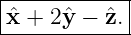
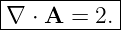
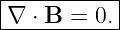
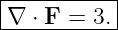
This companion article provides self-study exercises for EM03, Spatial Derivatives of fields:
gradient, divergence, and curl. All exercises are stated first. Complete worked solutions follow in
Part II.
The goal is not only to compute formulas mechanically, but also to connect each differential
operator with its physical meaning:
- the gradient of a scalar field points in the direction of fastest increase,
- the divergence of a vector field measures local source or sink strength, and
- the curl of a vector field measures local oriented circulation.
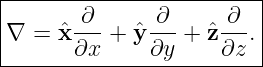
The central definitions used throughout are
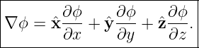
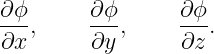
For a scalar field ϕ(x,y,z),
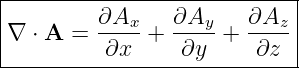
For a vector field A = Axx + Ayy + Azz,
and
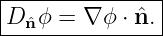
The directional derivative of a scalar field in the unit direction n is
For plane-wave phase,
so that
These are the same conventions developed in EM03 and in standard references on vector calculus
and electrodynamics [1, 2, 3, 4].
How to use this problem set
Attempt all exercises in Part I before reading Part II. For each answer, keep three questions
separate:
- What is the operator acting on?
- What kind of object should the result be: scalar or vector?
- What local physical or geometric meaning does the result have?
Many mistakes in vector calculus are not arithmetic errors but type errors: for example, expecting
a scalar from a gradient or expecting a vector from a divergence.
Part I: Exercises
Exercise 1: partial derivatives of a scalar field
Let
Compute
Exercise 2: gradient at a point
Let
Find:
- ∇ϕ;
- ∇ϕ at the point (1,−1, 2);
- the magnitude |∇ϕ| at that point;
- the unit direction of fastest increase at that point.
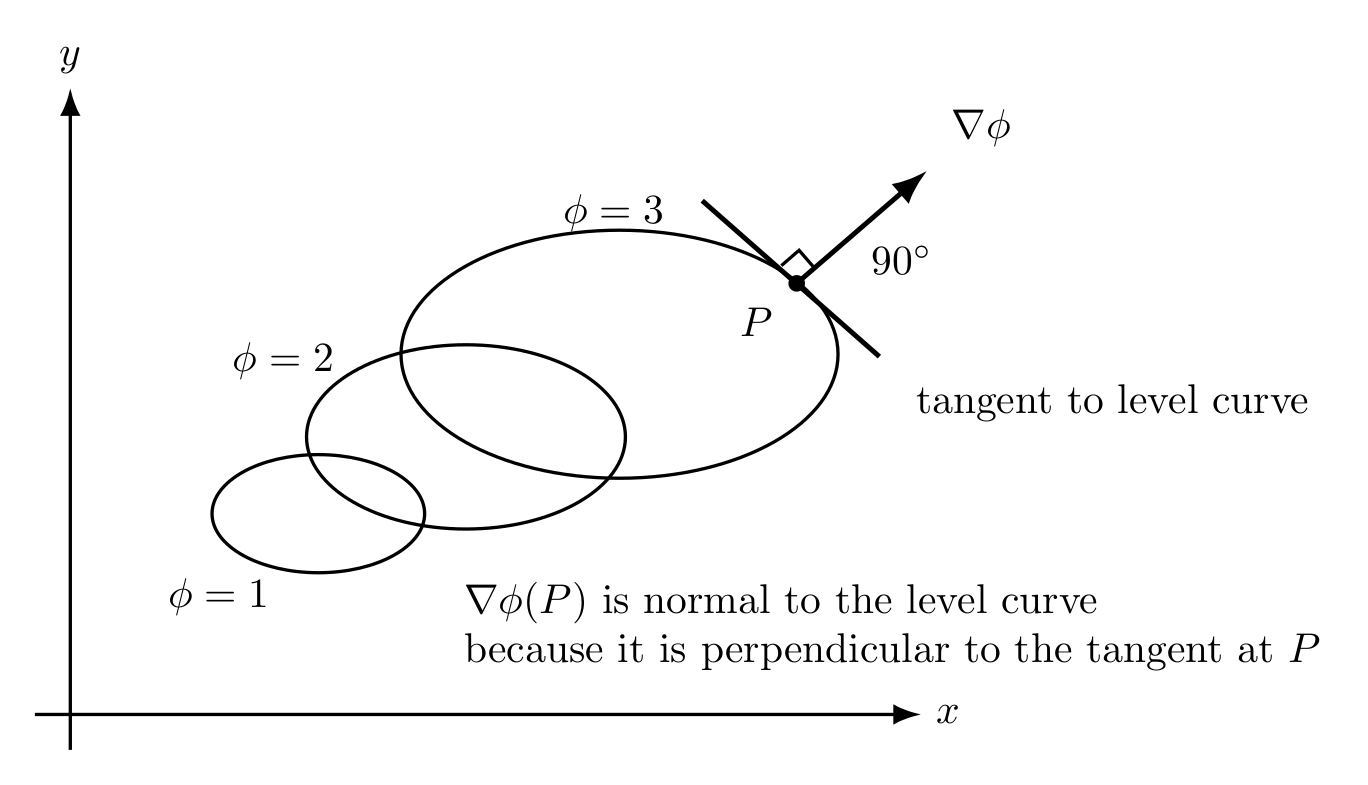
Figure. The gradient is normal to level curves and points toward larger scalar-field values.
Exercise 3: directional derivative
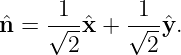
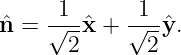
Using the scalar field from Exercise 2, find the directional derivative at (1,−1, 2) in the unit
direction
Interpret the sign of the result.
Exercise 4: level surfaces and normals
Consider the scalar field
Show that the surfaces ϕ = C are planes. Find a normal vector to these planes and explain its
relation to the gradient.
Exercise 5: divergence of a linear field
Let
Compute ∇⋅ A and state whether the field behaves locally like a net source, a net sink, or
neither.
Exercise 6: zero-divergence field
Let
Compute ∇⋅ B and interpret the result physically.
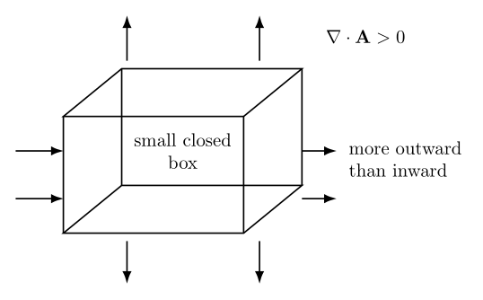
Figure. Divergence compares local outward and inward flux through a small closed box.
Exercise 7: divergence as flux density
A vector field is
At the point (1, 2, 0):
- compute ∇⋅ F;
- estimate the net outward flux through a small rectangular box of volume
centered at that point using the local relation
Exercise 8: curl of a rotational field
Let
Compute ∇× C.
Exercise 9: curl of a gradient field
Let
and let
Find G and then compute ∇× G.
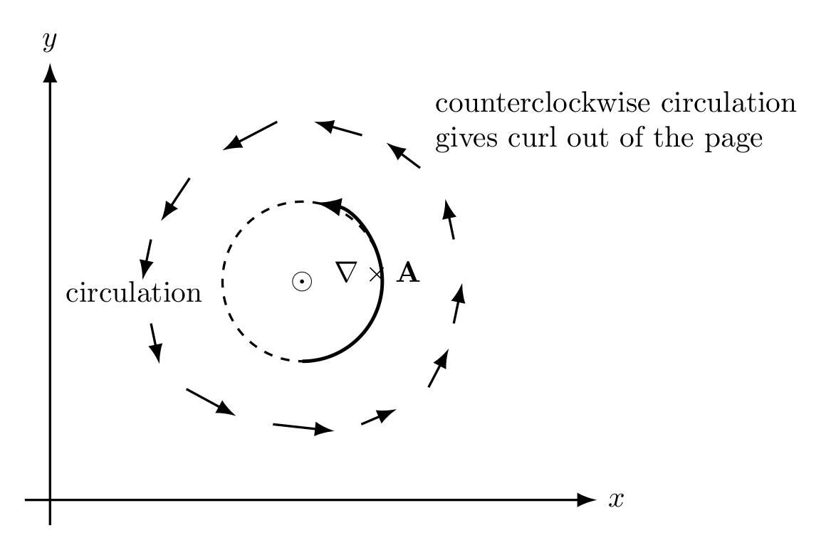
Figure. Curl measures the oriented circulation tendency around a small loop.
Exercise 10: compare zero divergence and zero curl
For the two vector fields
and
compute both ∇⋅ and ∇× for each field. Which field is source-like? Which field is rotational?
Exercise 11: gradient of plane-wave phase
Let the phase be
Find:
- ∇𝜃;
- the wave vector k;
- the magnitude |k|.
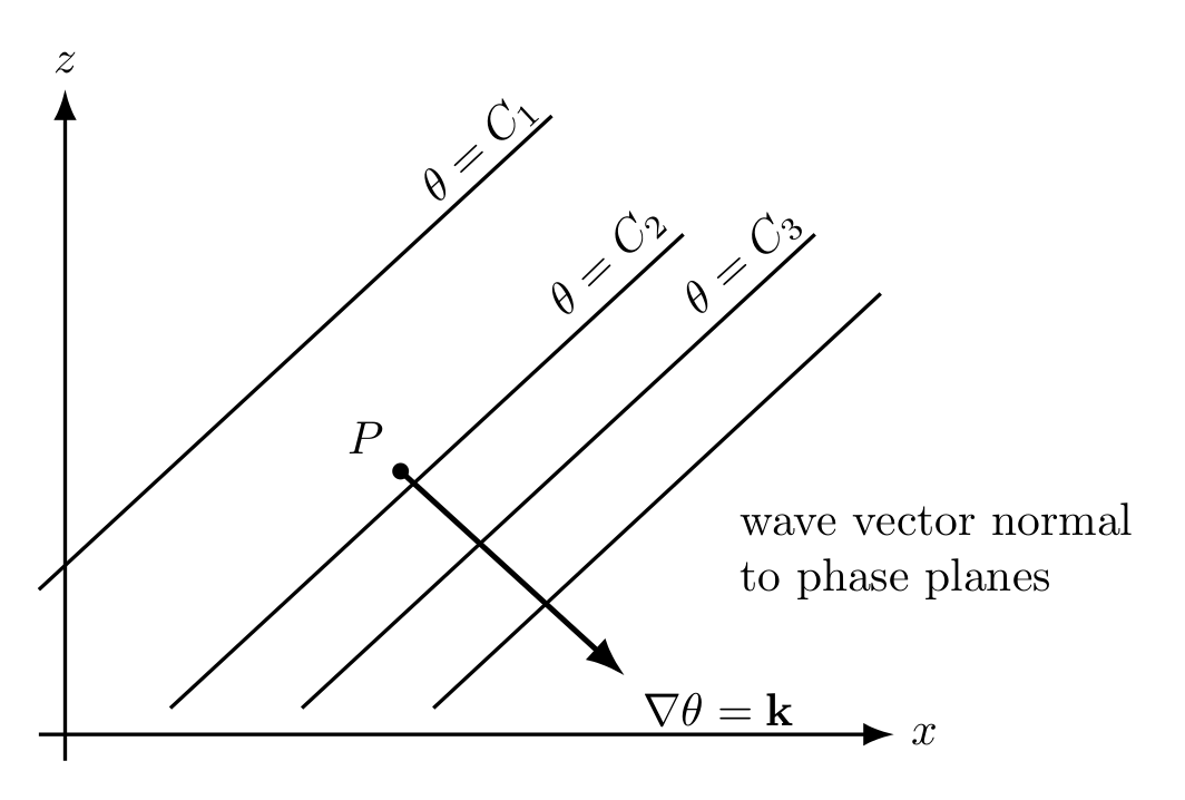
Figure. For a plane wave, the gradient of phase is the wave vector, normal to
constant-phase planes.
Exercise 12: gradient of a scalar plane wave
Let
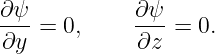
Treat this as a three-dimensional scalar field that depends only on x.
Find:
- ∂ψ∕∂x;
- ∇ψ;
- the direction of ∇ψ.
Exercise 13: divergence and curl of a transverse field
Let
Compute:
- ∇⋅ E;
- ∇× E.
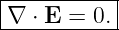
State clearly whether each result is zero or nonzero.
Exercise 14: identify the operator type and meaning
For each expression below, state whether the result is a scalar or a vector, and give its local
physical meaning.
- ∇ϕ;
- ∇⋅ A;
- ∇× A;
- ∇𝜃 for 𝜃 = k ⋅ r − ωt.
Part II: Complete worked solutions
Solution 1: partial derivatives of a scalar field
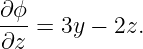
Given
we differentiate with respect to one variable at a time while holding the others fixed.
For x,
For y,
For z,
Therefore,
Solution 2: gradient at a point
The field is
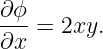
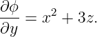
Its partial derivatives are
Hence
At (1,−1, 2),
Its magnitude is
Thus
The unit direction of fastest increase is the normalized gradient:
Solution 3: directional derivative
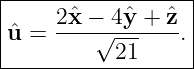
From Solution 2,
The unit direction is
Therefore,
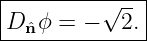
So
Thus
The negative sign means the scalar field decreases as one moves locally in the direction
n.
Solution 4: level surfaces and normals
If
then the level surfaces ϕ = C satisfy
which is the equation of a plane.
The gradient is
Therefore a normal vector to the level planes is
This illustrates the general rule that the gradient is normal to a constant-value surface.
Solution 5: divergence of a linear field
For
we identify
Then
Hence
Because the divergence is positive, the field behaves locally like a net source.
Solution 6: zero-divergence field
For
the components are
Therefore,
So
The field has no local net source or sink strength, even though it may still circulate.
Solution 7: divergence as flux density
Given
we compute
Thus,
Since the field is linear, this value is the same at (1, 2, 0).
Using
with ΔV = 0.02 m3, we obtain
Therefore,
in the corresponding flux units of the field.
Solution 8: curl of a rotational field
Let
Then
Using the component formula for curl,
The first two components are zero. The third is
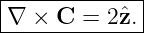
Hence
So the field has nonzero local circulation about the z axis.
Solution 9: curl of a gradient field
Given
its gradient is
Now compute the curl:
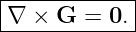
Every derivative above is zero, so
This is a standard example that a gradient field is irrotational.
Solution 10: compare zero divergence and zero curl
First consider
Its divergence is
Its curl is
Thus
So U is source-like but not rotational.
Now consider
Its divergence is
Its curl is
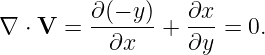
Therefore,
So V is rotational but not source-like.
Solution 11: gradient of plane-wave phase
For
we compute
Hence
By comparison with 𝜃 = k ⋅ r − ωt, we identify
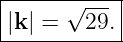
Its magnitude is
Thus
Solution 12: gradient of a scalar plane wave
Let
Differentiate with respect to x:
Because the field depends only on x,
Therefore,
So the gradient points purely in the ±x direction, depending on the sign of the sine
factor.
Solution 13: divergence and curl of a transverse field
The field is
Its components are
For the divergence,
Since Ex depends on z but not on x, and Ey = Ez = 0,
For the curl, only the y component survives. More explicitly,
However, from the standard component formula,
Thus,
and therefore
So the divergence is zero while the curl is generally nonzero.
Solution 14: identify the operator type and meaning
- ∇ϕ is a vector. It points in the direction of fastest increase of the scalar field and has
magnitude equal to the maximum local rate of increase.
- ∇⋅ A is a scalar. It measures local source or sink strength, or equivalently the net
outward flux per unit volume in the small-volume limit.
- ∇×A is a vector. It measures local oriented circulation, with the direction set by the
right-hand rule.
- ∇𝜃 is a vector. For plane-wave phase 𝜃 = k⋅r−ωt, it equals the wave vector k, which
is normal to constant-phase planes and points in the propagation direction.
Concluding remarks
The key lesson from EM03 and EM03E is that three different questions about spatial change lead
to three different operators:
asks how a scalar field rises,
asks whether a vector field spreads out or converges, and
asks whether a vector field circulates.
For plane-wave phase,
connects vector calculus directly to wave geometry.
The next lesson, EM04, combines these ideas further by introducing the Laplacian and the
three-dimensional wave equation.
References
[1] H. M. Schey, Div, Grad, Curl, and All That, 4th ed., W. W. Norton & Company,
2005.
[2] David J. Griffiths, Introduction to Electrodynamics, 4th ed., Cambridge University
Press, 2017.
[3] Gilbert Strang and Edwin “Jed” Herman, Calculus, Volume 3, OpenStax, 2016,
chapters on vector fields and vector calculus.
[4] Massachusetts Institute of Technology, 18.02SC Multivariable Calculus, MIT
OpenCourseWare, materials on gradient, divergence, curl, flux, and line integrals.
[5] Samuel J. Ling, Jeff Sanny, and William Moebs, University Physics, Volume 2,
OpenStax, 2016, chapters on electric and magnetic fields and electromagnetic waves.
[6] Richard P. Feynman, Robert B. Leighton, and Matthew Sands, The Feynman Lectures
on Physics, Volume II, Addison-Wesley, 1964, chapters on vector electromagnetic fields
and Maxwell’s equations.

![[parent]](https://images.physicslibrary.org/images/uparrow.png)