Electromagnetic Waves, Antennas, and RF: Vector Fields for Wave Mechanics
EM01 introduced the idea that Electromagnetism is naturally written in the language of fields. A
scalar field assigns one number to every point in space and time, while a vector field assigns a
vector. The next step is to make that vector language precise enough that later electromagnetic
equations can be read without ambiguity.
This article therefore develops only the vector mathematics needed immediately for wave
mechanics:
Gradient, divergence, curl, and Maxwell’s equations are intentionally deferred. The
purpose of EM02 is to establish the algebra and geometry that those later ideas will use
[1, 2, 3, 4].
1 One vector versus a vector field
A single vector might be written
It has a magnitude and a direction.
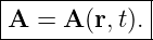
A vector field assigns such a vector to every point in space and time:
Using Cartesian coordinates,
so the field may also be written
The distinction is important:
- A can mean one particular vector;
- A(r,t) emphasizes that the vector can change from place to place and from time to
time.
For an electric field, for example,
returns one electric-field vector when a position and time are specified.
2 Cartesian basis vectors
In three-dimensional Cartesian coordinates, we use the unit basis vectors
Each has magnitude one:
They point in mutually perpendicular directions.
A vector may therefore be decomposed as
The quantities
are scalar components. They may be positive, negative, or zero.
The basis vectors carry the direction information.
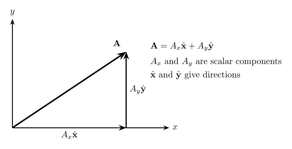
Figure. A vector can be reconstructed by adding its Cartesian component vectors. The
scalar numbers Ax and Ay specify signed amounts along the basis directions.
In two dimensions,
In three dimensions, the z component is added in exactly the same way.
3 Components can themselves be fields
For a vector field,
Each component is therefore a scalar field.
This point is extremely useful. A vector field can be viewed as three coupled scalar
fields:
For example,
has components
| Ex(z,t) | = E0 cos(kz − ωt), | (15)
|
| Ey(z,t) | = 0, | (16)
|
| Ez(z,t) | = 0. | (17) |
The field varies with z and t, but every field vector points along either +x or −x.
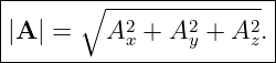
4 Magnitude of a vector
For
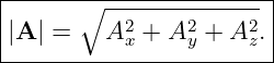
the magnitude is
This is the three-dimensional Pythagorean theorem.
The magnitude is never negative:
A negative component does not mean a negative magnitude. It means the vector points partly in
the negative direction of that coordinate axis.
5 Unit vector in an arbitrary direction
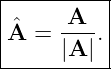
Suppose A≠0. Dividing the vector by its magnitude produces a unit vector pointing in the same
direction:
By construction,
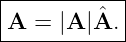
Therefore every nonzero vector can be written as
This separation into magnitude and direction will recur throughout electromagnetism.
6 The Cartesian basis is orthonormal
The word orthonormal combines two ideas:
- each basis vector has unit magnitude;
- different basis vectors are perpendicular.
Thus
while
The dot product makes these statements precise.
7 The dot product
For two vectors
and
the Cartesian dot product is
The result is a scalar.
The same dot product also has the geometric form
where 𝜃 is the angle between the vectors.
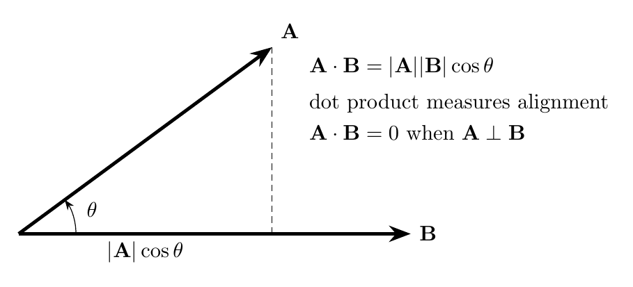
Figure. The dot product measures alignment. The factor |A| cos 𝜃 is the scalar projection
of A onto the direction of B when B is used only to define a direction.
8 Interpreting the sign of the dot product
Because
the sign tells us about relative orientation.
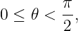
If
then
and the dot product is positive.
If
then
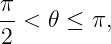
If
then the dot product is negative.
Thus the dot product provides a direct test for perpendicularity of nonzero vectors.
9 Projection onto a unit direction
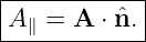
Let n be a unit vector. The scalar component of A along n is
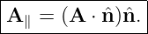
The corresponding vector projection is
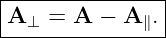
The part perpendicular to n is
This decomposition will later be useful for separating field components normal and tangential to
surfaces and for distinguishing polarization components.
10 The wave vector
The Wave Mechanics series used the scalar Wavenumber
In three dimensions we also need a propagation direction. We therefore define the wave
vector
where n points in the propagation direction.
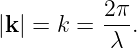
The magnitude is
The vector k therefore contains two pieces of information:
- its magnitude gives spatial phase rate;
- its direction gives the direction of propagation.
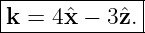
For propagation along +z,
11 Why the plane-wave phase contains a dot product
A three-dimensional plane-wave phase is written
To see why, write
and
Then
For a wave traveling only along +z,
so
The familiar one-dimensional phase
is therefore a special case of the three-dimensional phase.
12 Surfaces of constant phase
At a fixed time, points satisfying
for some constant C lie on a plane perpendicular to k.
Thus k is normal to a plane wavefront.
This will later make Huygens’ principle, apertures, phased arrays, and antenna far-field phase
much easier to express mathematically.
13 The cross product
The cross product of two vectors is another vector:
Its magnitude is
Its direction is perpendicular to both A and B.
The right-hand rule determines which of the two possible perpendicular directions is
chosen.
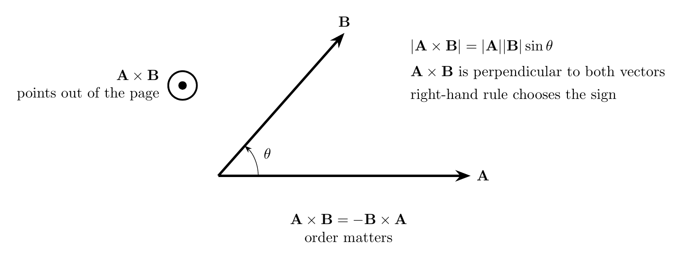
Figure. The cross product is perpendicular to the plane containing A and B. The
dot-in-circle symbol indicates a vector pointing out of the page.
14 Cross product in Cartesian components
For
and
the cross product is
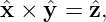
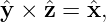
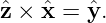
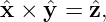
A useful memory pattern comes from the right-handed Cartesian basis:
Reversing the order changes the sign:
This is called anticommutativity.
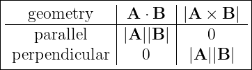
15 Parallel and perpendicular cases
If A and B are parallel, then
and
If they are perpendicular, then
and
The dot and cross products therefore respond differently to angle:
16 A first electromagnetic transverse triad
Later, Maxwell’s equations will show that an ideal uniform plane electromagnetic wave in a simple
isotropic medium has mutually perpendicular electric field, magnetic field, and propagation
direction.
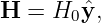
For the moment, we use that only as a geometric preview:
The dot-product tests are therefore
Their orientation also satisfies
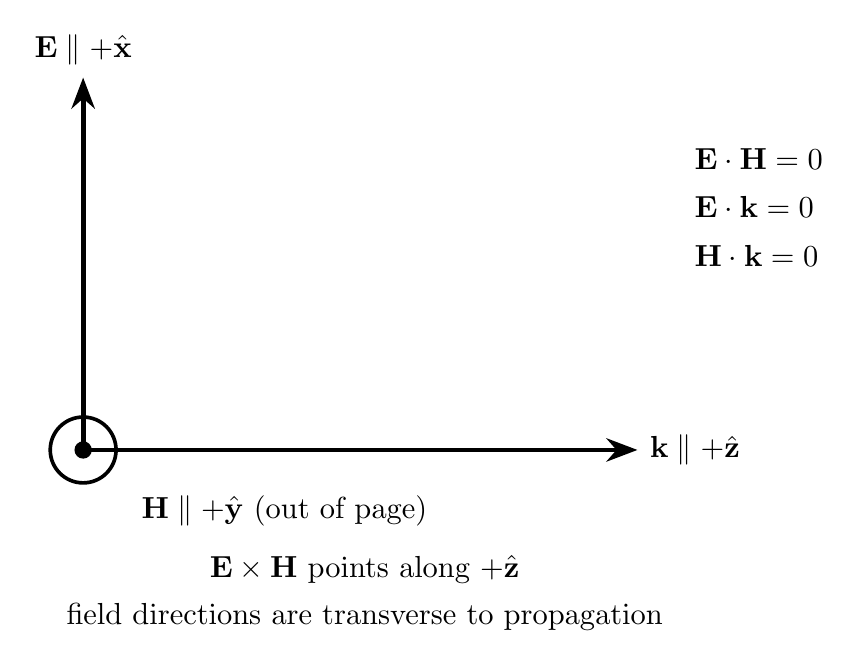
Figure. A right-handed transverse field triad. Here E points along +x, H points out of the
page along +y, and k points along +z. Detailed electromagnetic field relations are deferred;
EM02 uses this only to establish the geometry.
This geometry is central to radio waves. It will later connect the field vectors to energy transport
through the Poynting vector.
17 Field direction is not propagation direction
Consider
The vector x tells us the electric-field direction.
The phase
tells us the pattern propagates toward increasing z.
Therefore
For this example,
This distinction is one of the most important geometric habits to establish before studying
electromagnetic waves.
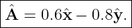
18 Worked Example 1: resolve a vector into components
Let
The components are
The negative y component means the vector points partly toward −y.
Its magnitude is
| |A| | = 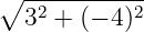 | (74)
|
| =  | (75)
|
| = 5. | (76) |
Thus
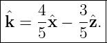
The corresponding unit vector is
So
19 Worked Example 2: dot product and perpendicularity
Let
and
Then
| A ⋅ B | = (2)(3) + (3)(−2) | (83)
|
| = 6 − 6 | (84)
|
| = 0. | (85) |
Therefore
We did not need to draw the vectors or explicitly compute the angle. The dot product provided the
test directly.
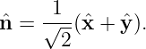
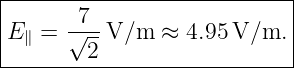
20 Worked Example 3: projection onto a measurement axis
Suppose
and a sensor measures only the component along
The scalar measured component is
| E∥ | = E ⋅n | (89)
|
| =  ⋅ ⋅  | (90)
|
| =  V/m. V/m. | (91) |
Therefore
The dot product extracts the part of the field aligned with the sensor axis.
21 Worked Example 4: evaluate a three-dimensional plane-wave phase
Let
and
Then
| k ⋅ r | = (2)(4) + (0)(1) + (3)(5) | (95)
|
| = 8 + 15 | (96)
|
| = 23 rad. | (97) |
Thus the spatial phase at that point is
The absent y component of k means displacement along y does not change the phase in this
example.
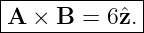
22 Worked Example 5: compute a cross product
Let
and
Using
we obtain
| A × B | = (2)(3)(x ×y) | (102)
|
| = 6z. | (103) |
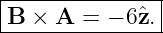
Therefore
Reversing the order gives
23 Worked Example 6: verify a transverse triad
Suppose
and
The dot products are
and
Thus the three directions are mutually perpendicular.
The cross product is
| E × H | = E0H0x ×y | (112)
|
| = E0H0z. | (113) |
Therefore
24 Worked Example 7: identify field and propagation directions
Consider
The electric field points along
The spatial phase is
Therefore
Its magnitude is
The propagation unit vector is
Finally,
so the electric field is transverse to the propagation direction.
25 Common mistakes
- Mistake: treating Axx as the same thing as the scalar Ax. One is a vector component
contribution; the other is a scalar coefficient.
- Mistake: assuming a negative component means a negative magnitude. Magnitude is
nonnegative; component signs encode direction.
- Mistake: confusing k with k. The scalar k is the magnitude of the wave vector, while
k also contains propagation direction.
- Mistake: forgetting that a dot product produces a scalar while a cross product
produces a vector.
- Mistake: assuming the cross product is commutative. Reversing the order reverses the
sign.
- Mistake: confusing field direction with propagation direction. A transverse wave can
propagate in one direction while its field vectors point in perpendicular directions.
- Mistake: using the plane-wave relation E ⊥ H ⊥ k as though it described every
electromagnetic field everywhere. EM02 uses it only as a preview of the ideal uniform
plane-wave geometry that will be derived later.
26 What EM02 adds to the field picture
EM01 introduced
as a vector-valued field.
EM02 now gives that notation operational meaning:
with magnitude
The dot product measures alignment and projection:
The cross product measures oriented perpendicular geometry:
The three-dimensional plane-wave phase becomes
And the electromagnetic-wave geometry we will later derive is summarized by
EM03 next uses this vector foundation to introduce spatial derivatives of fields: gradient,
divergence, and curl.
References
[1] David J. Griffiths, Introduction to Electrodynamics, 4th ed., Cambridge University
Press, 2017.
[2] Samuel J. Ling, Jeff Sanny, and William Moebs, University Physics, Volume 2,
OpenStax, 2016, chapters on electric and magnetic fields and electromagnetic waves.
[3] Richard P. Feynman, Robert B. Leighton, and Matthew Sands, The Feynman
Lectures on Physics, Volume II, Addison-Wesley, 1964, chapters introducing vector
electromagnetic fields.
[4] Massachusetts Institute of Technology, 8.02 Physics II: Electricity and Magnetism,
MIT OpenCourseWare, materials on vector fields and electromagnetic phenomena.
[5] H. M. Schey, Div, Grad, Curl, and All That, 4th ed., W. W. Norton & Company,
2005.
[6] Frank S. Crawford, Jr., Waves, Berkeley Physics Course, Volume 3, McGraw-Hill,
1968.