1.1. Classical Mechanics. In classical mechanics, we study the motion of a particle. This motion
is described by a (vector) function of one variable, q = q(t), representing the position of
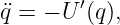
the particle as a function of time. This function must satisfy the Newton equation of
motion,
where U the potential energy, and the mass of the particle is 1. Another way to express this law of
motion is to say that q(t) must be a solution of a certain variational problem. Namely, one
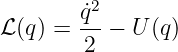
introduces the Lagrangian
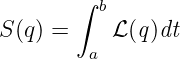
(the difference of kinetic and potential energy), and the action functional
(for some fixed a < b). Then the law of motion can be expressed as the least action principle: q(t)
must be a critical point of S on the space of all functions with given q(a) and q(b). In other words,
the Newton equation is the Euler-Lagrange equation for the solution of the variational problem
defined by S.
Remark 1. The name “least action principle” comes from the fact that in some cases (for example
when U′′ ≤ 0) the action is not only extremized but also minimized at the solution q(t). In general,
however, it is not the case, and the trajectory of the particle may not be a minimum, but only a
saddle point of the action. Therefore, the law of motion is better formulated as the
“extremal (or stationary) action principle” ; this is the way we will think of it in the
future.
Remark 2. Physicists often consider solutions of Newton’s equation on the whole line rather than
on a fixed interval [a, b]. In this case, the naive definition of an extremal does not make sense,
since the action integral S(q) = ∫
ℝℒ(q)dt is improper and in general diverges. Instead, one
makes the following “correct” definition: a function q(t) on ℝ is an extremal of S if the
expression
where 𝜖(t) is any compactly supported perturbation, is identically zero. With this definition, the
extremals are exactly the solutions of Newton’s equation.
1.2. Classical field theory. In classical field theory, the situation is similar. In this case, we
should think not of a single particle, but of a “continuum of particles” (e.g. a string, a membrane,
a jet of fluid); so the motion is described by a classical field-a (vector) function ϕ(x, t) depending
on both space and time coordinates (x ∈ ℝd, t ∈ ℝ). Consequently, the equation of motion is a
partial differential equation. For example, for a string or a membrane the equation of
motion is the wave equation □ϕ = 0, where □ is the D’Alembertian ∂t2 − v2△ (here
△ is the Laplacian with respect to the space coordinates, and v the velocity of wave
propagation).
As in mechanics, in classical field theory there is a Lagrangian ℒ(ϕ) (a differential polynomial in
ϕ), whose integral S(ϕ) = ∫
Dℒ(ϕ)dxdt over a region D in space and time is called the
action. The law of motion can be expressed as the condition that the action must be
extremized over any closed region D and fixed boundary conditions; so the equations
of motion (also called the field equations) are the Euler-Lagrange equations for this
variational problem. For example, in the case of string or membrane, the Lagrangian
is
Remark. Like in mechanics, solutions of the field equations on the whole space (rather than a
closed region D) are extremals of the action in the sense that
where 𝜖 is a compactly supported perturbation.
1.3. Brownian motion. One of the main differences between classical and quantum mechanics is,
roughly speaking, that quantum particles do not have to obey the classical equations of motion,
but can randomly deviate from their classical trajectories. Therefore, given the position and
velocity of the particle at a given time, we cannot determine its position at a later time, but can
only determine the density of probability that at this later time the particle will be found at a
given point. In this sense quantum particles are similar to random (Brownian) particles.
Brownian particles are a bit easier to understand conceptually, so let us begin with
them.
The motion of a Brownian particle in ℝd in a potential field U : ℝd → ℝ is described by astochastic
process q = q(t), q = (q1, …, qd) ∈ ℝd. That is, for each real t we have a random variable q(t)
(position of the particle at a time t), such that the dependence of t is regular in some sense.
The random dynamics of the particle is “defined” as follows: 1 if y : [a, b] → ℝd is a
continuously differentiable function, then the density of probability that q(t) = y(t) for
t ∈ [a, b] is proportional to e−S(y)∕κ, where S(y) := ∫
ab( y′2 − U(y))dt is the action for the
corresponding classical mechanical system, and κ is the diffusion coefficient. Thus, for
given q(a) and q(b), the likeliest q(t) is the one that minimizes S (in particular, solves
the classical equations of motion q = −U′(q)), while the likelihood of the other paths
decays exponentially with the deviation of the action of these paths from the minimal
possible.
y′2 − U(y))dt is the action for the
corresponding classical mechanical system, and κ is the diffusion coefficient. Thus, for
given q(a) and q(b), the likeliest q(t) is the one that minimizes S (in particular, solves
the classical equations of motion q = −U′(q)), while the likelihood of the other paths
decays exponentially with the deviation of the action of these paths from the minimal
possible.
Remark. This discussion assumes that the extremum of S at q is actually a minimum, which we
know is not always the case.
All the information we can hope to get about such a process is contained in the correlation
functions < qi1(t1)…qin(tn) >, which by definition are the expectation values of the products of
random variables qi1(t1)…qin(tn) (more specifically, by Kolmogorov’s theorem the stochastic process
q(t) is completely determined by these functions). So such functions should be regarded as the
output, or answer, of the theory of the Brownian particle.
So the main question is how to compute the correlation functions. The definition above obviously
gives the following answer: given t1, …, tn ∈ [a, b], we have
where integration is carried out over the space of paths [a, b] → ℝn, and Dq is a Lebesgue
measure on the space of paths such that ∫
e−S(q)∕κDq = 1. Such an integral is called a path
integral, since it is an integral over the space of paths.
It is clear, however, that such definition and answer are a priori not satisfactory from the
mathematical viewpoint, since the infinite dimensional integration that we used requires
justification. In this particular case, such justification is possible within the framework of Lebesgue
measure theory, and the corresponding integration theory is called the theory of Wiener integrals.
(To be more precise, one cannot define the measure Dq, but one can define the measure e−S(q)∕κDq
for sufficiently nice potentials U(q)).
1.4. Quantum mechanics. Now let us turn to a quantum particle. Quantum mechanics is
notoriously difficult to visualize, and the randomness of the behavior of a quantum particle is less
intuitive and more subtle than that of a Brownian particle; nevertheless, it was pointed out by
Feynman that the behavior of a quantum particle in a potential field U(q) is correctly described by
the same model, with the real positive parameter κ replaced by the imaginary number iℏ, where
ℏ > 0 is the Planck constant. In other words, the dynamics of a quantum particle can be expressed
via the correlation functions
where Dq is normalized so that ∫
eiS(q)∕ℏDq = 1.
1.5. Quantum field theory. The situation is the same in field theory. Namely, a useful theory of
quantum fields (used in the study of interactions of elementary particles) is obtained when one
considers correlation functions
where Dϕ is normalized so that ∫
eiS(ϕ)∕ℏDϕ = 1.
Of course, from the mathematical point of view, this setting is a priori even less satisfactory than
the one for the Brownian particle, since it involves integration with respect to the complex valued
measure eiS(q)∕ℏDq, which nobody knows how to define. Nevertheless, physicists imagine that
certain integrals of this type exist and come to correct and interesting conclusions (both physical
and mathematical). Therefore, making sense of such integrals is an interesting problem for
mathematicians.
References
This is a derivative work from [1] a Creative Commons Attribution-Noncommercial-Share Alike 3.0
work
[1] MIT OpenCourseWare, 18.238 Geometry and Quantum Field Theory, Fall 2002