FS02: Inner Products of Functions
FS01 showed that a complicated periodic waveform can be assembled from harmonics. The next
question is more precise:
- How can we measure how much of one candidate harmonic is contained in a function?
The answer begins with ordinary vector geometry.
For a vector, the dot product measures alignment and extracts components. Fourier analysis uses
the same geometric idea, but the “vectors” are functions and the dot product becomes an
integral.
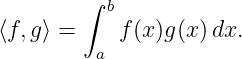
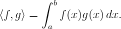
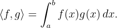
The central definition of this lecture will be
This lecture develops Equation (1) slowly rather than treating it as a mysterious rule. We will
build it from:
- ordinary vector dot products,
- orthogonality,
- vector projection,
- the passage from finite sums to integrals,
- function norms and normalization,
- projection of one function onto another,
- residual orthogonality,
- weighted inner products.
The trigonometric orthogonality identities themselves are postponed to FS03. By the end of FS02,
however, the reason Fourier coefficients are projection coefficients should already be
clear.
1 Review: the dot product of ordinary vectors
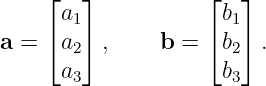
Consider two vectors in three-dimensional Euclidean space:
Their dot product is
This operation takes two vectors and returns one scalar.
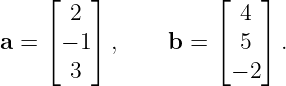
For example, let
Then
| a ⋅ b | = (2)(4) + (−1)(5) + (3)(−2) | (5)
|
| = 8 − 5 − 6 | (6)
|
| = −3. | (7) |
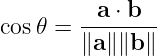
The dot product contains geometric information. It can be written as
where 𝜃 is the angle between the vectors.
Thus:
- a positive dot product indicates an acute angle,
- a negative dot product indicates an obtuse angle,
- a zero dot product indicates a right angle.
2 Orthogonal vectors
Two nonzero vectors are orthogonal when
From Equation (8),
If both vectors are nonzero, their norms are nonzero, so
Therefore
Orthogonality is therefore the general algebraic form of perpendicularity.
3 Projection of one vector onto another
Suppose we want the part of v that points along a nonzero vector e.
Any vector parallel to e has the form
for some scalar c.
We therefore write
where r is the leftover or residual vector.
For ce to be the projection, the residual should contain no component along e. Therefore
require
Substitute
Then
Distribute the dot product:
Move the second term to the other side:
Divide by e ⋅ e:
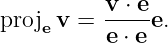
Thus the projection itself is
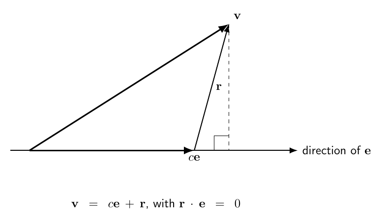
Figure 1. Vector projection. The coefficient multiplying e is chosen so that the residual r = v − ce
is perpendicular to e. This same residual-orthogonality idea will be reused for functions.
4 Special case: projection onto a unit vector
If e is a unit vector, then
Equation (20) becomes
This is why components in an orthonormal Cartesian basis are obtained by dot products.
For example,
Fourier analysis will eventually do the same thing with normalized basis functions.
5 From vectors to lists of sampled function values
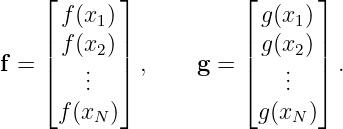
Suppose we sample two functions f and g at equally spaced points
The function values form lists:
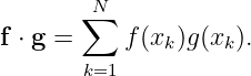
An ordinary discrete dot product is
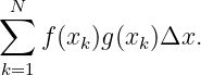
If the points have spacing Δx, multiply by Δx:
Equation (28) is a Riemann sum. As the sample spacing becomes smaller and the number of
samples increases, the sum approaches an integral:
This provides a natural bridge from the finite-dimensional vector dot product to a continuous
function inner product.
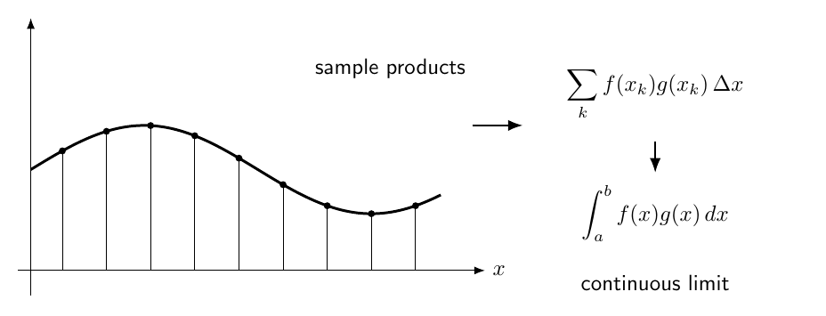
Figure 2. A function inner product can be motivated by sampling two functions, multiplying
corresponding samples, summing them, and then taking the continuous limit of the weighted sum.
6 Definition of the inner product of real functions
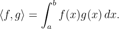
For real-valued functions on the interval [a,b], define
The angle brackets distinguish the function inner product from ordinary multiplication.
It is important to read the notation correctly:
is one number obtained from two entire functions.
The integration interval is part of the definition. The same pair of functions can be orthogonal on
one interval and not orthogonal on another.
7 Property 1: symmetry
For real functions,
Because multiplication of real numbers is commutative,
Therefore
| ⟨f,g⟩ | = ∫
abf(x)g(x) dx | (34)
|
| = ∫
abg(x)f(x) dx | (35)
|
| = ⟨g,f⟩. | (36) |
Thus
8 Property 2: linearity
Let α and β be constants. Then
| ⟨αf + βh,g⟩ | = ∫
ab[αf(x) + βh(x)]g(x) dx | (38)
|
| = α∫
abf(x)g(x) dx + β ∫
abh(x)g(x) dx | (39)
|
| = α⟨f,g⟩ + β⟨h,g⟩. | (40) |
So the inner product is linear in each argument for real-valued functions.
9 Property 3: positivity
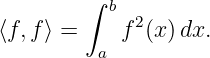
Take the inner product of a function with itself:
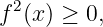
Because
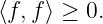
we have
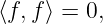
For the ordinary function spaces used in this series, if
then f is zero except possibly on sets that do not affect the integral. For elementary continuous
functions, this simply means
throughout the interval.
10 Norm of a function
The Euclidean vector norm satisfies
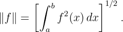
The analogous function norm is
Therefore
The norm measures the overall size of the function over the interval.
It does not generally equal the maximum value of the function. It is an integrated measure of
magnitude.
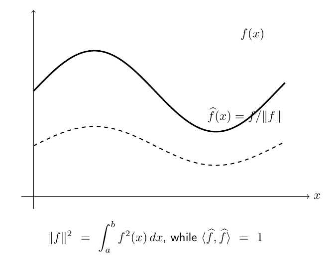
Figure 3. The function norm is determined by the area under f2(x), not by the largest single
value of f. Normalizing a function rescales its entire graph so that its inner product with itself
equals one.
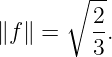
11 Example: norm of f(x) = x on [−1, 1]
Let
Then
| ∥f∥2 | = ⟨f,f⟩ | (50)
|
| = ∫
−11x2 dx. | (51) |
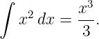
An antiderivative is
Thus
| ∥f∥2 | =  −11 | (53)
|
| =  −  | (54)
|
| =  . | (55) |
Therefore
12 Normalization of a function
A normalized function has norm one.
Given a nonzero function f, define
Then
| ⟨f,f⟩ | = 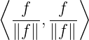 | (58)
|
| =  ⟨f,f⟩ | (59)
|
| = 1. | (60) |
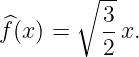
For f(x) = x on [−1, 1],
13 Orthogonal functions
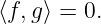
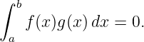
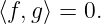
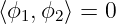
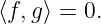
Two functions are orthogonal on [a,b] when
In integral form,
The functions do not need to look geometrically perpendicular on an ordinary graph. The word
orthogonal refers to their inner product.
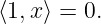
14 Example: 1 and x on [−1, 1]
Let
Then
| ⟨1,x⟩ | = ∫
−11xdx | (65)
|
| =  −11 | (66)
|
| =  −  | (67)
|
| = 0. | (68) |
Therefore 1 and x are orthogonal on [−1, 1].
The cancellation occurs because x is negative on the left half and positive on the right
half.
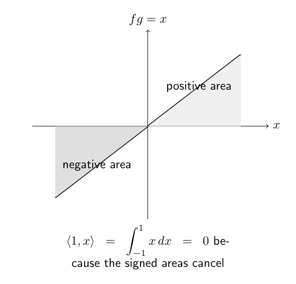
Figure 4. Orthogonality of 1 and x on a symmetric interval. Their product is just x, whose
negative and positive signed areas cancel exactly over [−1,1].
15 The interval matters
Use the same functions on [0, 1]:
| ⟨1,x⟩ | = ∫
01xdx | (69)
|
| =  01 | (70)
|
| =  . | (71) |
Now the inner product is not zero.
Therefore:
- 1 and x are orthogonal on [−1, 1],
- 1 and x are not orthogonal on [0, 1].
Orthogonality belongs to the functions together with the chosen inner product and
interval.
16 Even and odd symmetry already helps
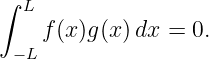
Suppose f is even and g is odd on the symmetric interval [−L,L].
Then
and
Their product satisfies
| [fg](−x) | = f(−x)g(−x) | (74)
|
| = f(x)[−g(x)] | (75)
|
| = −f(x)g(x). | (76) |
Thus fg is odd.
The integral of an odd function over a symmetric interval is zero:
Therefore every even function is orthogonal to every odd function under this standard inner
product on a symmetric interval, provided the integral exists.
This symmetry observation will save substantial work later.
17 Projection of one function onto another
Now repeat the vector argument using functions.
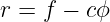
Suppose we want to approximate f(x) using one nonzero function ϕ(x). Write
where r is the residual.
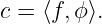
For cϕ to contain all of the component of f along ϕ, require the residual to be orthogonal to
ϕ:
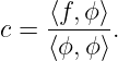
From Equation (78),
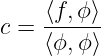
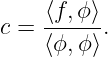
Therefore
Use linearity:
Thus
Finally,
This is one of the central equations of the Fourier-series learning path.
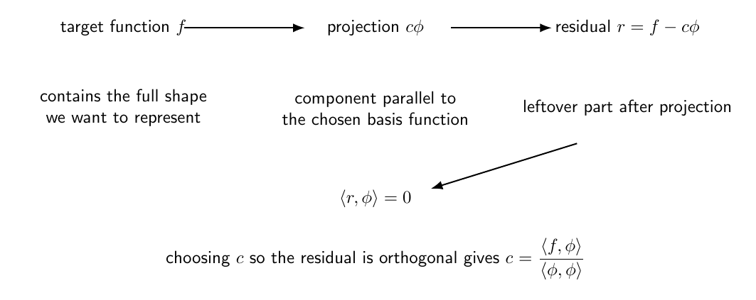
Figure 5. Function projection uses the same geometry as vector projection. The coefficient c is
selected so that the residual r = f − cϕ has zero inner product with the basis function ϕ.
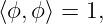
18 If the basis function is normalized
If
then Equation (84) simplifies to
This is the function-space analogue of taking the dot product with a unit vector.
19 Worked projection example: approximate x2 by a constant
Let
on [−1, 1].
Approximate it using the constant basis function
We seek
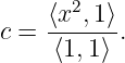
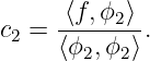
The projection coefficient is
Compute the numerator:
| ⟨x2, 1⟩ | = ∫
−11x2 dx | (91)
|
| =  . | (92) |
Compute the denominator:
| ⟨1, 1⟩ | = ∫
−111 dx | (93)
|
| = 2. | (94) |
Therefore
| c | =  | (95)
|
| =  . | (96) |
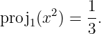
So the projection of x2 onto the constant functions is
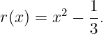
The residual is
Check its orthogonality to the constant basis:
| ⟨r, 1⟩ | = ∫
−11 dx | (99)
|
| =  −  (2) | (100)
|
| = 0. | (101) |
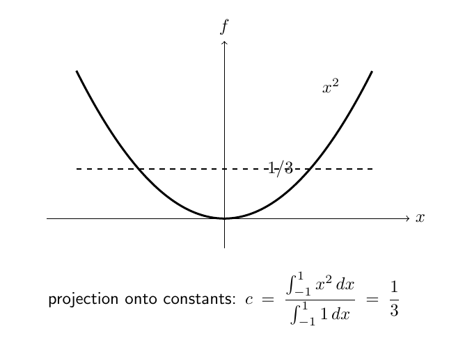
Figure 6. Projection of x2 onto the constant basis function on [−1,1]. The best constant
projection in the inner-product sense is 1∕3, leaving a residual whose signed integral is zero.
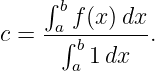
20 Why the projection constant equals the average value
For the constant basis function ϕ = 1 on [a,b],
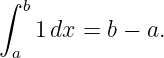
But
Therefore
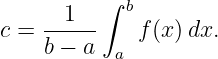
Equation (104) is exactly the average value of f over the interval.
Thus the average or DC component of a function can be understood geometrically as its projection
onto the constant function.
This observation will later explain the constant term in a Fourier series.
21 Projection onto several orthogonal functions
Suppose
are mutually orthogonal:
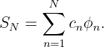
Approximate f by
Require the residual
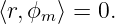
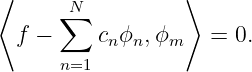
be orthogonal to every basis function:
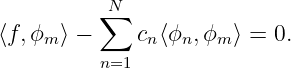
Substitute the residual:
Use linearity:
Because the functions are orthogonal, every term with
vanishes. Only the n = m term remains:
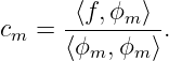
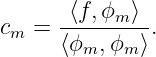
Therefore
This is the general projection formula behind real Fourier coefficients.
FS03 will establish that the sine and cosine functions used in Fourier series are orthogonal on the
appropriate interval. Once that is known, Equation (114) will immediately tell us how to isolate
one harmonic.
22 Orthonormal functions
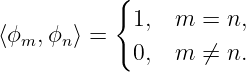
A collection of functions is orthonormal when
This combines two properties:
- different basis functions are orthogonal,
- each basis function has norm one.
For an orthonormal basis, Equation (114) simplifies to
This is the cleanest analogue of Cartesian vector components.
23 Pythagorean relation for orthogonal functions
For orthogonal functions f and g,
Compute the squared norm of their sum:
| ∥f + g∥2 | = ⟨f + g,f + g⟩ | (118)
|
| = ⟨f,f⟩ + ⟨f,g⟩ + ⟨g,f⟩ + ⟨g,g⟩. | (119) |
The cross terms vanish:
Therefore
Equation (121) is the function-space Pythagorean theorem.
Later, Parseval’s theorem will be an infinite-dimensional version of this idea.
24 Angle between functions
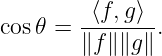
The vector relation
suggests an analogous definition for nonzero real functions:
This provides a geometric interpretation of the inner product.
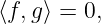
If
then
so the functions can be regarded as separated by a 90∘ angle in function space.
The graph of one function is not literally drawn at right angles to the graph of the other. The
angle belongs to the abstract geometry defined by the inner product.
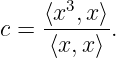
25 Worked example: project x3 onto x
On [−1, 1], let
We seek
The coefficient is
The numerator is
| ⟨x3,x⟩ | = ∫
−11x4 dx | (129)
|
| =  −11 | (130)
|
| =  −  | (131)
|
| =  . | (132) |
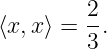
The denominator is
Thus
| c | =  | (134)
|
| =   | (135)
|
| =  . | (136) |
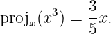
Therefore the projection is
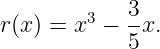
The residual is
Check orthogonality:
| ⟨r,x⟩ | = ∫
−11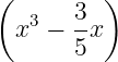 xdx | (139)
|
| = ∫
−11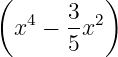 dx | (140)
|
| =  −   | (141)
|
| =  −  | (142)
|
| = 0. | (143) |
26 Weighted inner products
The ordinary inner product treats every point of the interval with the same Weight.
Sometimes a problem naturally assigns greater importance to some parts of the interval than
others.
Define a weighted inner product by
where the weight function satisfies
throughout the interval, apart from possible special endpoint behavior in more advanced
settings.
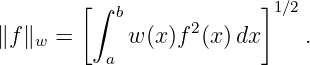
The associated weighted norm is
Weighted inner products will become important later in generalized eigenfunction expansions and
Sturm-Liouville theory.
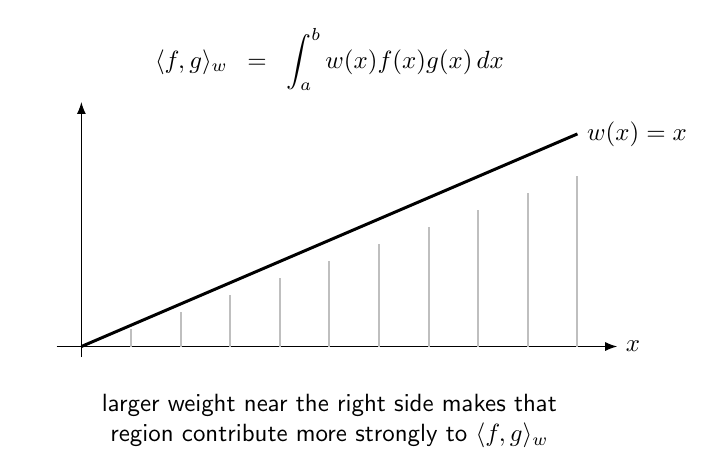
Figure 7. A weighted inner product changes how strongly different portions of the interval
contribute. Regions with larger w(x) influence the projection and norm more strongly.
27 Example of a weighted projection
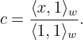
On [0, 1], let
The weighted projection coefficient onto the constant function is
Compute the numerator:
| ⟨x, 1⟩w | = ∫
01(2x)(x)(1) dx | (149)
|
| = 2 ∫
01x2 dx | (150)
|
| =  . | (151) |
The denominator is
| ⟨1, 1⟩w | = ∫
012xdx | (152)
|
| = 1. | (153) |
Thus
Without the weight, the ordinary average of x on [0, 1] is
The weight w = 2x emphasizes the right side of the interval, where x is larger, so the weighted
projection shifts upward to 2∕3.
28 Units of a function inner product
Suppose f and g have physical units [f] and [g], and x has units [x].
Then
Therefore an inner product is not necessarily dimensionless.
Likewise,
In mathematical treatments, variables are often nondimensionalized or the units are suppressed. In
physics applications, the dimensions should still be checked.
29 Function space: what does it mean to treat a function like a vector?
A vector in ordinary three-dimensional space is specified by three components. A function requires
infinitely many values to specify its complete shape.
The phrase function space refers to a set of functions treated as points or vectors in a larger
abstract space.
The inner product supplies geometry to that space. It lets us define:
- length through ∥f∥,
- orthogonality through ⟨f,g⟩ = 0,
- angle through Equation (123),
- projection through Equation (84).
This geometric viewpoint is the foundation of Fourier analysis.
A rigorous treatment eventually introduces Hilbert spaces and equivalence classes of functions.
That level of functional analysis is not needed yet. The elementary integral geometry is enough to
derive Fourier series.
30 Why orthogonality makes coefficient extraction easy
Suppose
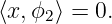
Take the inner product with ϕ2:
| ⟨f,ϕ2⟩ | = ⟨c1ϕ1 + c2ϕ2 + c3ϕ3,ϕ2⟩ | (159)
|
| = c1⟨ϕ1,ϕ2⟩ + c2⟨ϕ2,ϕ2⟩ + c3⟨ϕ3,ϕ2⟩. | (160) |
If the basis functions are mutually orthogonal,
and
Therefore
Hence
The inner product with ϕ2 destroys every orthogonal component and leaves only the ϕ2
component.
This is exactly what FS04 and FS05 will do with cosine and sine harmonics.
31 Preview of the Fourier connection
FS01 introduced a finite harmonic sum of the form
If the functions
are orthogonal over one full period, then each coefficient can be extracted by projection.
For example, the structure must look like
The proportionality factor depends on the norm of the cosine basis function.
We are not yet entitled to write the final Fourier coefficient formula because we have not proved
the required trigonometric orthogonality identities.
That is the purpose of FS03.
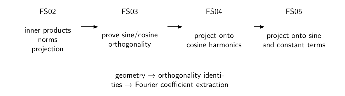
Figure 8. FS02 supplies the geometry. FS03 will prove that distinct sine and cosine harmonics are
orthogonal, after which FS04 and FS05 can extract individual Fourier coefficients by projection.
32 A first three-function orthogonal example
On [−1, 1], consider
We already know
Now check
| ⟨1,ϕ2⟩ | = ∫
−11 dx | (170)
|
| =  −  | (171)
|
| = 0. | (172) |
Next,
| ⟨x,ϕ2⟩ | = ∫
−11x dx | (173)
|
| = ∫
−11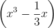 dx. | (174) |
The integrand is odd, so
Thus the three functions are mutually orthogonal.
This example illustrates a general strategy: new basis functions can be constructed by
subtracting projections onto earlier basis functions. A systematic version of this process is the
Gram-Schmidt procedure, which will be useful later but is not needed for the first Fourier
derivations.
33 Self-check questions
- What does the inner product of two functions return: another function or a scalar?
- Why is the integration interval part of the definition of orthogonality?
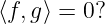
- What does it mean geometrically if
- Derive the projection coefficient
from residual orthogonality.
- Why does the denominator disappear for a normalized basis function?
- What is the projection of a function onto the constant basis function physically related
to?
- Why does an even function have zero inner product with an odd function over a symmetric
interval?
- Why does orthogonality make it possible to isolate one coefficient from an expansion
containing many coefficients?
- What is the difference between an orthogonal set and an orthonormal set?
- Why are we postponing the Fourier coefficient formulas until after FS03?
34 Practice problems
- Compute
on [−1, 1].
- Determine whether x and x2 are orthogonal on [−1, 1].
- Determine whether 1 and x are orthogonal on [−2, 2] and on [0, 2].
- Compute the norm of f(x) = 1 on [−L,L].
- Normalize f(x) = 1 on [−L,L].
- Compute the norm of f(x) = x on [−2, 2].
- Project f(x) = x2 onto the constant function on [0, 1].
- Project f(x) = x4 onto the constant function on [−1, 1].
- Project f(x) = x3 onto ϕ(x) = x on [−2, 2].
- Show directly that x2 − 1∕3 is orthogonal to 1 on [−1, 1].
- Suppose ϕ1 and ϕ2 are orthogonal. Prove
- Using the weighted inner product with w(x) = x on [0, 1], project f(x) = x onto the constant
function.
35 Summary
The ordinary vector dot product
has a continuous analogue for real functions:
This inner product defines the geometry needed for Fourier analysis.
Two functions are orthogonal when
The norm of a function is
The projection coefficient of f onto a nonzero basis function ϕ is
This coefficient is obtained by requiring the residual
be orthogonal to ϕ.
For an orthogonal collection {ϕn},
FS03 now supplies the missing ingredient: it proves in detail that distinct sine and cosine
harmonics are orthogonal over a complete period.
References
References
[1] PhysicsLibrary, FS00: Fourier Series Roadmap, Motivation, and Learning Path.
[2] PhysicsLibrary, FS01: Periodic Functions, Harmonics, and Why Fourier Series Exist.
[3] E. Kreyszig, Advanced Engineering Mathematics, Wiley.
[4] G. B. Arfken, H. J. Weber, and F. E. Harris, Mathematical Methods for Physicists,
Academic Press.