|
|
|
|||||||
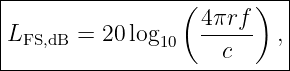
For free space,
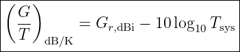
while
and
Use
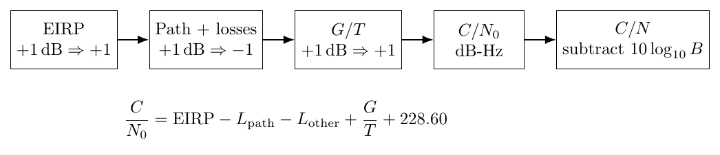
Figure. End-to-end sensitivity chain. A one-decibel change in any additive dB budget term produces a one-decibel change in C∕N0 with the sign shown, while bandwidth enters only when converting C∕N0 to C∕N.
Part I: Exercises
Exercise 1: baseline end-to-end RF linkA telemetry transmitter operates at 2.20 GHz over a 250 km free-space path. The transmitter power is 10.0 dBW, transmit feeder loss is 1.50 dB, transmit antenna gain is 12.0 dBi, and all other propagation/implementation losses total 2.50 dB. The receive antenna gain is 8.00 dBi, the system noise temperature is 500 K, and the receiver noise-equivalent bandwidth is 1.00 MHz. Find (a) EIRP, (b) free-space path loss, (c) received carrier power, (d) G∕T, (e) C∕N0, and (f) C∕N.
Exercise 2: vary range while everything else is fixedRepeat Exercise 1 after the range doubles from 250 km to 500 km. Determine the change in free-space path loss and C∕N0. If the minimum required C∕N0 is 75.0 dB-Hz, compute the link margin before and after the range change.
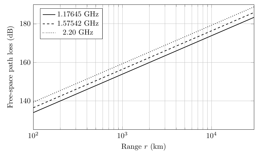
Figure. Free-space path loss grows by 20 log 10r and 20 log 10f. Doubling either range or frequency increases FSPL by 6.02 dB when antenna gains are held fixed.
Exercise 3: vary frequency at fixed antenna gainsReturn to the 250 km geometry of Exercise 1, but double the carrier frequency from 2.20 GHz to 4.40 GHz. Hold all antenna gains, EIRP, losses, and receiver noise quantities fixed. Find the new FSPL and C∕N0. Explain why this fixed-gain comparison is not the same as holding physical antenna aperture fixed.
Exercise 4: compensate range loss with EIRPFor the 500 km case of Exercise 2, determine the EIRP required to restore the original 250 km value of C∕N0. If antenna gain and transmit feeder loss remain unchanged, find the required transmitter power in dBW and watts. Compare with the original 10 W transmitter.
Exercise 5: trade receive gain against system temperatureStarting from Exercise 1, compare two independent receiver improvements:
Find the new G∕T and the improvement in C∕N0 for each case.
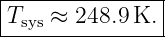
Exercise 6: system-temperature degradationStarting from Exercise 1, suppose environmental or front-end conditions increase Tsys from 500 K to 1000 K while all gains and losses remain fixed. Calculate the new G∕T and C∕N0. Show that doubling system temperature causes approximately a 3.01 dB penalty.
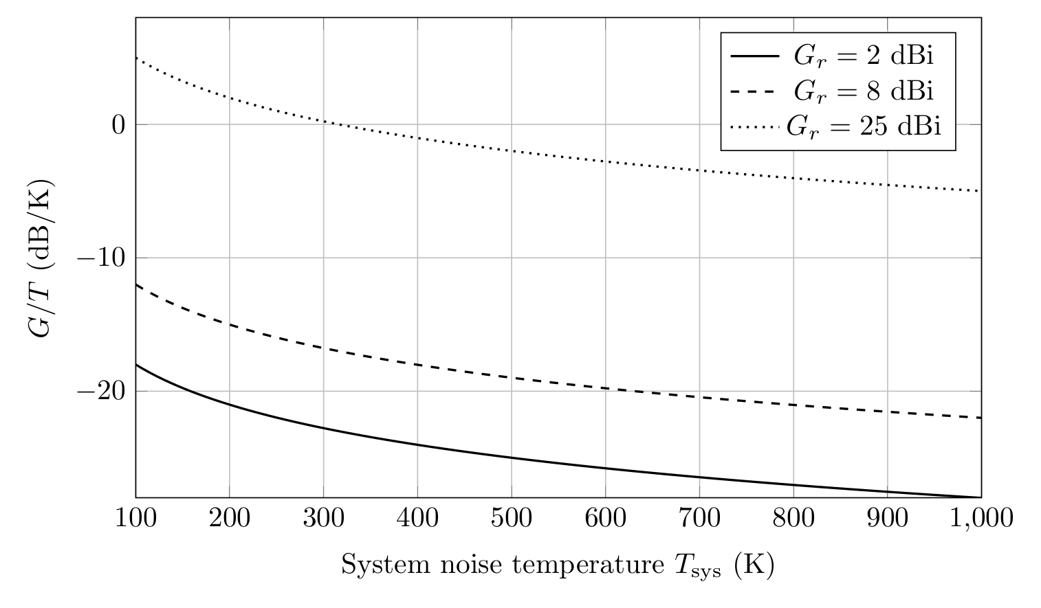
Figure. Receiver G∕T versus system noise temperature for several receive gains. Increasing antenna gain moves the entire curve upward; reducing temperature moves the operating point to the left.
Exercise 7: bandwidth sweepThe baseline link in Exercise 1 has a fixed C∕N0. Compute C∕N for noise-equivalent bandwidths of 100 kHz, 1.00 MHz, and 10.0 MHz. Explain why C∕N0 does not change when the receiver bandwidth is changed in this idealized calculation.
Exercise 8: increase miscellaneous lossesThe baseline link uses Lother = 2.50 dB. In an adverse condition suppose the combined atmospheric, polarization, pointing, radome, and implementation losses rise to 6.00 dB. Recalculate C∕N0 and the margin relative to a 75.0 dB-Hz requirement. How much margin was consumed solely by the additional losses?
Exercise 9: nominal GNSS-style end-to-end budgetConsider an illustrative L1-like link with
Find FSPL, received carrier power, G∕T, C∕N0, and C∕N in a 2.00 MHz front-end bandwidth. If the receiver requires 42.0 dB-Hz, find the nominal C∕N0 margin.
Exercise 10: GNSS-style range variationKeep all Exercise 9 quantities fixed except range, which increases from 20,200 km to 26,000 km. Determine the additional path loss, the new C∕N0, and the new margin relative to 42.0 dB-Hz.
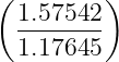
Exercise 11: GNSS-style frequency comparison at fixed gainsUsing the Exercise 9 range and all other quantities fixed, compare f1 = 1.57542 GHz with f2 = 1.17645 GHz. Calculate the FSPL at the lower frequency and the change in C∕N0. State clearly the assumption that antenna gains, rather than physical apertures, are being held fixed.
Exercise 12: reference-plane synthesis with feed loss and LNA noiseAt the antenna terminals, the antenna noise temperature is 100 K. A 1.00 dB passive feed loss at 290 K precedes an LNA with 0.80 dB noise figure. The receive antenna gain is 25.0 dBi. (a) Refer the feed and LNA noise temperatures back to the antenna-terminal plane and find Tsys. (b) Find G∕T. (c) For a link with EIRP = 15.0 dBW, Lpath = 180 dB, and Lother = 2.00 dB, find C∕N0 and C∕N in 1.00 MHz. Explain why the 1 dB feed loss must not be subtracted again if its effect has already been included consistently in the quoted G∕T.
Exercise 13: receiver degradation from noise-like interferenceFor the GNSS-style link of Exercise 9, suppose an admitted noise-like interferer has
Use
to find the degradation in dB, the degraded effective C∕N0, and the remaining margin above a 42.0 dB-Hz threshold.
Exercise 14: allowable interference density from marginFor the same nominal GNSS-style link, use the clean-link margin to determine the maximum J0∕N0 that can be admitted before the effective C∕N0 reaches the 42.0 dB-Hz threshold under the additive noise-like interference model. Use
where M is the clean-link margin in dB.
Exercise 15: why J∕S is not the same as degradationFor Exercise 9, the carrier power is C and the system temperature is 400 K. Suppose the noise-like interference density is again J0∕N0 = −8.00 dB and the receiver bandwidth is 2.00 MHz. Find (a) N0 in dBW/Hz, (b) J0 in dBW/Hz, (c) total in-band J in dBW, (d) J∕S in dB, and (e) the additive-power degradation. Explain why a positive J∕S can coexist with less than 1 dB of degradation in this example.
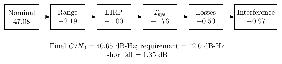
Figure. Example margin waterfall. Independent degradations subtract from the clean-link C∕N0 margin; noise-like interference enters through its nonlinear degradation 10 log 10(1 + J0∕N0).
Exercise 16: combined worst-case sensitivity and recoveryStart with the nominal GNSS-style C∕N0 from Exercise 9. Now apply all of the following changes simultaneously:
Find the final effective C∕N0 and margin relative to 42.0 dB-Hz. If only one scalar budget term can be improved, determine the minimum improvement in EIRP or G∕T required to restore the threshold.
Part II: Complete Worked Solutions
Solution 1: baseline end-to-end RF linkThe EIRP is
Thus
The free-space path loss is
Hence
The received carrier power at the antenna-terminal reference plane is
Therefore
The receiver figure of merit is
Thus
Now
Therefore
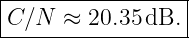
For Bn = 1.00 MHz,
Hence
Solution 2: vary range while everything else is fixedDoubling range gives
The new FSPL is
Because no other term changes, C∕N0 falls by the same amount:
The original margin above 75.0 dB-Hz was
while at 500 km
Thus
A factor of two in range consumed just over 6 dB of link margin.
Solution 3: vary frequency at fixed antenna gainsAt fixed range,
Therefore
and
This result assumes the quoted transmit and receive gains remain fixed. If physical antenna aperture were held fixed instead, antenna gain would generally increase with frequency, and part or all of the apparent 20 log 10f penalty could be offset. The comparison must therefore state what antenna property is held constant.
Solution 4: compensate range loss with EIRPThe doubled range added
of path loss. To restore the original C∕N0, EIRP must increase by the same amount:
With the original Lt = 1.50 dB and Gt = 12.0 dBi,
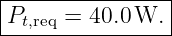
The corresponding power is
Thus
Doubling range requires four times the transmitter power if gain and every other term remain fixed, which is the inverse-square law expressed in power-budget form.
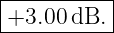
Solution 5: trade receive gain against system temperatureFor the gain improvement,
Compared with the original −18.990 dB/K, the improvement is exactly
Therefore C∕N0 also improves by 3.00 dB. For the temperature improvement,
The improvement is
Hence
A 3 dB gain increase and a factor-of-two temperature reduction are nearly equivalent in this scalar link budget.
Solution 6: system-temperature degradationWith Tsys = 1000 K,
Thus
The new carrier-to-noise-density ratio is
Therefore
The penalty is
which follows directly from 10 log 10(1000∕500) = 3.010 dB.
Solution 7: bandwidth sweepThe carrier-to-noise-density ratio remains
For 100 kHz,
For 1.00 MHz,
For 10.0 MHz,
Hence
for 100 kHz, 1 MHz, and 10 MHz respectively. C∕N0 is a carrier-power-to-noise-density quantity and therefore does not depend on the later choice of integrated noise bandwidth in this ideal model.
Solution 8: increase miscellaneous lossesThe loss increase is
Thus C∕N0 decreases by 3.50 dB:
The remaining margin above 75.0 dB-Hz is
The additional losses consumed exactly
of margin because dB losses enter the budget linearly.
Solution 9: nominal GNSS-style end-to-end budgetThe free-space path loss is
Thus
The carrier power is
Therefore
The receiver figure of merit is
Hence
The density ratio is
Thus
For Bn = 2.00 MHz,
Therefore
The clean-link C∕N0 margin is
Solution 10: GNSS-style range variationThe new FSPL at 26,000 km is
The increase is
Therefore
The remaining margin is
Solution 11: GNSS-style frequency comparison at fixed gainsAt 1.17645 GHz and the same 20,200 km range,
Relative to 1.57542 GHz, the reduction is
With EIRP, receive gain, losses, and system temperature held fixed, C∕N0 increases by the same amount:
Again, this is a fixed-gain comparison. If the physical antenna aperture were fixed, gain would itself vary with frequency.
Solution 12: reference-plane synthesis with feed loss and LNA noiseConvert the 1.00 dB feed loss to a linear power loss:
The feed equivalent input noise temperature is
The LNA noise factor is
so
Because the LNA follows the lossy feed, its noise referred to the antenna-terminal plane is multiplied by Lf:
Thus
The figure of merit is
Hence
The end-to-end density ratio is
Therefore
For 1.00 MHz,
The feed loss has already affected the receiver through the input-referred system temperature used in G∕T. Subtracting the same loss again from the compact C∕N0 equation would double-count it unless the reference plane were redefined consistently.
Solution 13: receiver degradation from noise-like interferenceConvert the interference ratio to linear form:
The degradation is
Therefore
The effective density ratio is
The remaining margin is
Solution 14: allowable interference density from marginThe clean-link margin is
Hence
Therefore
This is a receiver tolerance result under the stated additive noise-like interference model. It is not a statement that every interference waveform with the same total power will produce identical degradation.
Solution 15: why J∕S is not the same as degradationAt 400 K,
Thus
Since J0∕N0 = −8.00 dB,
Across 2.00 MHz,
So
The carrier from Exercise 9 is
therefore
Yet the relevant noise-like interference ratio is only J0∕N0 = −8 dB, which gives
The positive J∕S compares integrated interference power with the weak carrier. The degradation model instead compares interference spectral density with thermal-noise density. The bandwidth and spectral distribution therefore matter; J∕S alone is not sufficient to predict receiver degradation.
Solution 16: combined worst-case sensitivity and recoveryStart from
The range change from 20,200 km to 26,000 km costs
The EIRP reduction costs
The temperature increase from 400 K to 600 K costs
The extra miscellaneous loss costs
For J0∕N0 = −6 dB,
The final effective value is therefore
Thus
Relative to the 42.0 dB-Hz requirement,
The link is short by 1.351 dB. Therefore a single scalar improvement of at least
in EIRP or G∕T would restore the threshold under this model. The same deficit could also be recovered by an equivalent reduction in modeled losses or by some combination of smaller improvements.
Summary of sensitivity rulesThese problems expose several recurring link-budget scalings:
References
References
[1] H. T. Friis, “A Note on a Simple Transmission Formula,” Proceedings of the IRE, vol. 34, no. 5, pp. 254–256, 1946. [2] D. M. Pozar, Microwave Engineering, 4th ed., Wiley, 2012. [3] C. A. Balanis, Antenna Theory: Analysis and Design, 4th ed., Wiley, 2016. [4] E. D. Kaplan and C. J. Hegarty, eds., Understanding GPS/GNSS: Principles and Applications, 3rd ed., Artech House, 2017. [5] J. W. Betz, Engineering Satellite-Based Navigation and Timing: Global Navigation Satellite Systems, Signals, and Receivers, Wiley-IEEE Press, 2016. "example of Electromagnetic Waves, Antennas, and RF: End-to-End RF and GNSS Link-Budget Synthesis" is owned by bloftin.
This object's parent. Cross-references: units, noise factor, carrier-to-noise-density ratio, scalar, clean-link margin, noise figure, noise temperature, temperature, system, carrier frequency, antenna gain, power, relation, system noise temperature, free-space path loss, physical quantity, EM28 This is version 1 of example of Electromagnetic Waves, Antennas, and RF: End-to-End RF and GNSS Link-Budget Synthesis, born on 2026-10-10. Object id is 1462, canonical name is ExampleOfElectromagneticWavesAntennasAndRFEndToEndRFAndGNSSLinkBudgetSynthesis. Accessed 11 times total. Classification:
|
|
|
|
Pending Errata and AddendaNone.
|
DiscussionNo messages.
|
Interact |
![[parent]](https://images.physicslibrary.org/images/uparrow.png)










![[4π (250 × 103)(2.20 × 10⁹ )]
--------------------8-----
2.99792458 × 10](https://images.physicslibrary.org/cache/objects/1462/make4ht/ExampleOfElectromagneticWavesAntennasAndRFEndToEndRFAndGNSSLinkBudgetSynthesis12x.png)






























![[4π (20,200 × 103 )(1.57542 × 10⁹ )]
--------------------------------
c](https://images.physicslibrary.org/cache/objects/1462/make4ht/ExampleOfElectromagneticWavesAntennasAndRFEndToEndRFAndGNSSLinkBudgetSynthesis46x.png)