Binary Stars as Physical Laboratories
A single star can reveal its spectrum, brightness, temperature, chemical composition, motion,
and sometimes its radius. Its mass, however, is usually inferred indirectly from stellar
models.
A binary star changes that situation.
Two stars in mutual orbit respond directly to gravity. Their changing positions, velocities, and
brightness can encode the masses, radii, inclination, luminosity ratio, eccentricity, and evolutionary
state of the system.
This is why binary stars are often described as physical laboratories for stellar astrophysics.
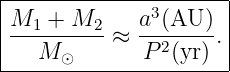
The central idea of this article is:
The most powerful systems combine several observing channels. A binary might be simultaneously
resolved on the sky, detected spectroscopically, and eclipsing.
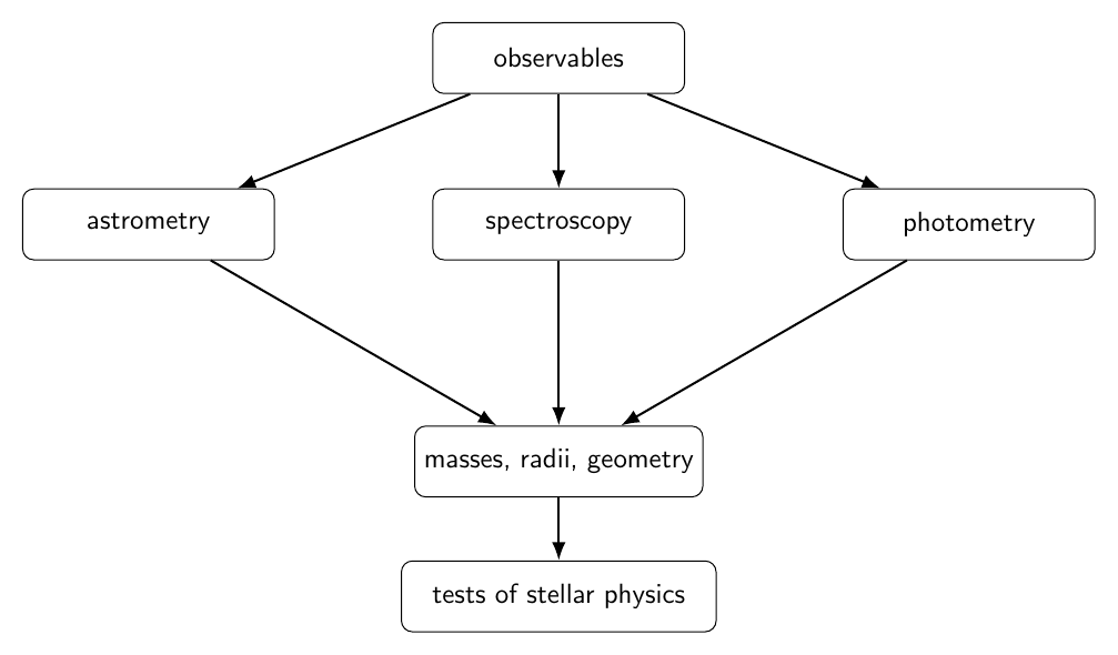
Figure 1. Binary stars connect directly observable quantities such as position, radial velocity, and
flux to stellar masses, radii, orbital geometry, and tests of stellar evolution.
1 What is a binary star?
A physical binary is a pair of stars that are gravitationally bound and orbit their common center of
mass.
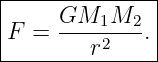
For stars of masses M1 and M2 with separation vector r, the two-body gravitational interaction is
described at first approximation by Newtonian gravity:
The same gravitational interaction causes each star to orbit the common center of mass.
A binary should be distinguished from an optical double. Two unrelated stars can lie nearly along
the same line of sight and therefore appear close together on the sky even though they are at very
different distances and are not gravitationally bound.
2 Physical pair versus optical double
A small angular separation alone does not prove that two stars form a bound system.
Evidence for a physical pair can include:
- common distance,
- common proper motion,
- orbital curvature in relative astrometry,
- compatible radial velocities,
- a complete orbital solution,
- eclipses or Doppler motion with a common period.
A chance alignment may show:
- very different parallaxes,
- inconsistent proper motions,
- no orbital motion despite a long observational baseline.
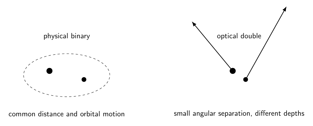
Figure 2. Two stars close together in angle can be either a gravitationally bound binary or an
optical double produced by line-of-sight projection. Distance and motion information help
distinguish the cases.
3 Observational classifications are not mutually exclusive
Binary stars are often classified by how they are detected.
This is an observational classification, not necessarily a unique physical class.
A single system can belong to several categories simultaneously.
3.1 Visual binary
A visual binary is resolved into two stellar images, and repeated relative astrometry can reveal
orbital motion.
The basic observables are often:
- angular separation,
- position angle,
- time.
3.2 Astrometric binary
An astrometric binary is recognized through periodic positional motion.
Sometimes only one component is directly measured. Sometimes the observable is the motion of
the photocenter rather than either star individually.
3.3 Spectroscopic binary
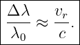
Orbital motion shifts spectral lines through the doppler effect.
For nonrelativistic radial velocities,
A system showing one moving spectrum is called single-lined, or SB1.
A system showing two moving spectra is called double-lined, or SB2.
3.4 Eclipsing binary
If the orbital plane is viewed sufficiently close to edge-on, one star can pass in front of the
other.
The measured brightness then shows periodic eclipses.
The system may also show ellipsoidal variation, reflection effects, starspots, or other variability
between eclipses.
3.5 Interacting and high-energy binaries
Some binaries are recognized through accretion, emission lines, X-rays, radio emission, outbursts,
or other signatures of mass exchange.
These physical phenomena are treated later in the BIN series.
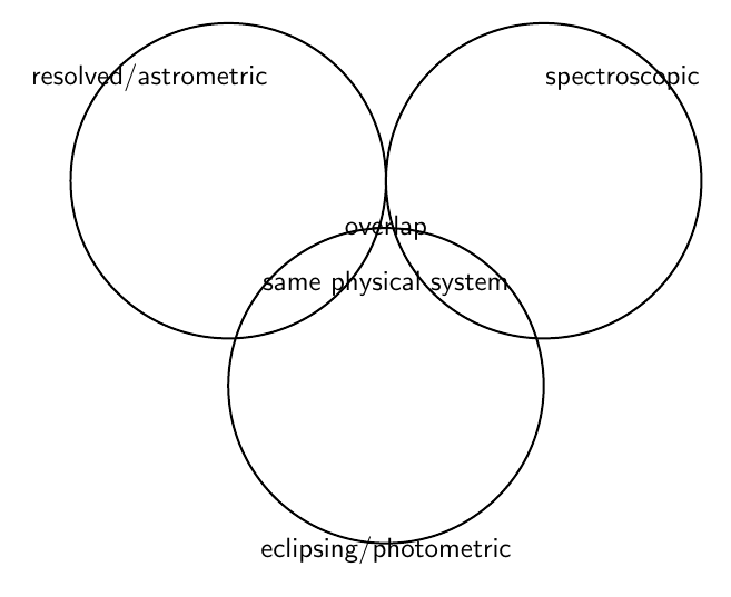
Figure 3. Visual, astrometric, spectroscopic, and eclipsing classifications describe observing
channels and can overlap in the same physical binary system.
4 Why multiple observing channels are powerful
Different observations constrain different parameters.
For example:
- sky-plane astrometry constrains the apparent orbit,
- parallax provides a distance scale,
- radial velocities measure line-of-sight orbital motion,
- eclipses constrain inclination and relative radii,
- spectra constrain temperature, surface gravity, and composition.
A system measured in only one channel can leave strong parameter degeneracies.
A system measured in several channels can break those degeneracies.
This principle is central to modern astrophysics:
5 Angular separation and physical scale
Astronomers initially observe angles on the sky, not distances between stars in meters or
astronomical units.
Suppose two stars have angular separation 𝜃 and are approximately at the same distance
d.
For a small angle,
where 𝜃 is measured in radians and s⊥ is the projected physical separation.
The word projected is essential. The actual three-dimensional separation can be larger.
6 The parsec and a useful binary star relation
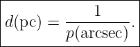
By definition, one parsec is the distance at which one astronomical unit subtends one
arcsecond.
Therefore a particularly useful astronomical form of the small-angle relation is
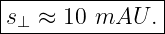
For example, a pair separated by
at
has projected separation
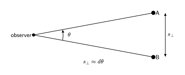
Figure 4. A measured angular separation becomes a projected physical separation once the
distance is known. In astronomy units, s⊥(AU) ≈ 𝜃(arcsec)d(pc).
7 Distance from parallax
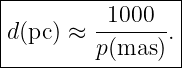
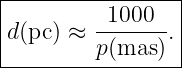
For a parallax p in arcseconds,
If parallax is given in milliarcseconds,
This simple inversion is appropriate for high signal-to-noise parallax measurements used in
introductory examples.
For low signal-to-noise or systematically uncertain parallaxes, distance inference becomes a
statistical problem and direct inversion can become biased. That issue is deferred to later methods
articles.
8 Projected separation is not the semimajor axis
A single measured sky separation should not be inserted directly into Kepler’s third law as though
it were automatically the orbital semimajor axis.
The observed separation depends on:
- orbital phase,
- eccentricity,
- inclination,
- argument and longitude of orientation,
- projection onto the sky.
The actual orbit requires repeated observations or another orbital constraint.
This distinction is one of the first important habits in binary star analysis:
9 Dynamical masses
Binary stars are especially valuable because gravity makes stellar mass measurable.
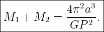
For a Keplerian binary with relative-orbit semimajor axis a and period P,
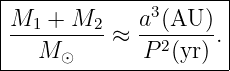
When a is in astronomical units, P is in years, and mass is in solar masses,
This form shows immediately why a physical length scale is required.
An angular orbit alone is not enough. A distance is also needed.
10 The center of mass and the mass ratio
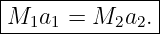
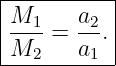
Let the stars have distances a1 and a2 from the center of mass.
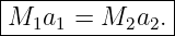
The center of mass relation is
Therefore
The more massive star moves on the smaller barycentric orbit.
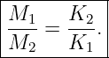
For a double-lined spectroscopic binary, the radial-velocity amplitudes carry the same inverse
mass-ratio information:
The full derivation is developed in BIN07.
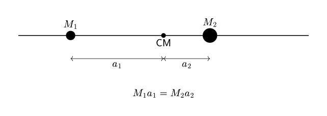
Figure 5. The center of mass divides the orbital scale inversely with stellar mass. The more
massive component has the smaller barycentric orbit.
11 Eclipses add geometric information
Eclipses occur only for favorable viewing orientations.
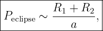
For a circular orbit, an order-of-magnitude geometric eclipse probability is
when
This relation already reveals an observational selection effect: close binaries are geometrically more
likely to eclipse than wide binaries.
If a system does eclipse, the light-curve geometry can constrain:
- orbital inclination,
- fractional stellar radii R1∕a and R2∕a,
- radius ratio,
- surface-brightness ratio,
- eccentricity information through eclipse timing and duration.
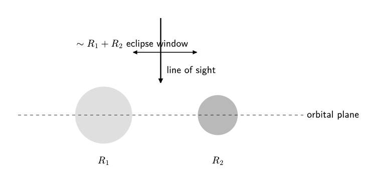
Figure 6. Eclipses require the projected orbital geometry to carry one star across the disk of the
other. The same geometry that enables eclipses also constrains inclination and relative stellar
radii.
12 Why eclipsing spectroscopic binaries are especially valuable
A spectroscopic orbit measures velocity information but usually contains factors of
where i is orbital inclination.
An eclipsing light curve constrains i geometrically.
Combining the two data types can therefore convert projected dynamical quantities into absolute
stellar masses and radii.
Detached eclipsing, double-lined systems are among the most important empirical calibrators of
stellar models because both stars can often be measured with relatively little complication from
mass transfer.
13 Binary stars test stellar evolution
The two stars in a binary usually formed together from the same natal environment.
To a useful approximation they therefore share:
- age,
- initial chemical composition,
- distance.
Yet they may have different masses.
That makes a binary a controlled experiment for stellar evolution.
A successful stellar model should be able to explain both components with one common age
and composition while reproducing their measured masses, radii, temperatures, and
luminosities.
BIN10 develops this idea in detail.
14 Binary stars test extreme physics
The same basic orbital framework extends to systems containing:
In these systems, binary dynamics can reveal an unseen compact object’s mass.
Interacting compact binaries can also probe:
- accretion physics,
- strong magnetic fields,
- thermonuclear outbursts,
- relativistic timing effects,
- gravitational-wave emission.
The sequence builds toward those applications gradually rather than treating them as isolated
topics.
15 Not every binary is easy to detect
Observed binary samples are shaped by selection effects.
A binary may be missed because:
- its angular separation is below the instrument resolution,
- its companion is much fainter than the primary,
- the orbit is too long compared with the observing baseline,
- its radial-velocity amplitude is too small,
- its orbital inclination suppresses the measured radial velocity,
- it does not eclipse,
- its variability is below photometric precision.
Therefore
without a model of detectability.
This becomes a major research topic in BIN23.
16 Resolution and contrast
Two stars can be physically widely separated yet difficult to resolve if they are distant.
Conversely, a nearby pair with small physical separation may be easily resolved.
Angular resolution is only one limitation.
Contrast also matters. A faint companion near a bright primary can be difficult to detect even
when the angular separation exceeds the nominal diffraction scale.
Binary star observations therefore combine:
- angular resolution,
- photometric contrast,
- signal-to-noise ratio,
- time baseline,
- cadence,
- spectral resolution.
17 From an observable to a stellar parameter
A useful mental map is:
| parallax | → distance, | (22)
|
| angular orbit + distance | → physical orbit, | (23)
|
| physical orbit + period | → total mass, | (24)
|
| two component orbits | → mass ratio, | (25)
|
| radial velocities | → line-of-sight orbital motion, | (26)
|
| eclipse morphology | → inclination and relative radii. | (27) |
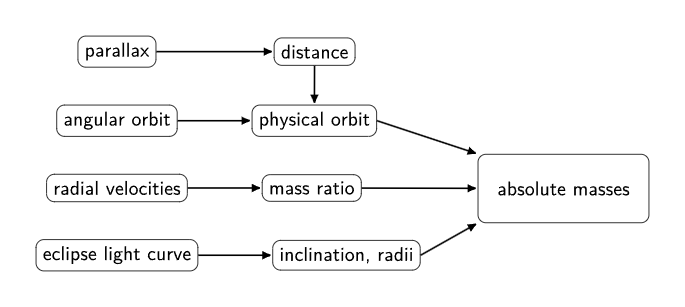
Figure 7. Different observable channels constrain complementary pieces of the binary star
problem. Combining them converts measured angles, velocities, times, and fluxes into physical
stellar parameters.
18 Hierarchical multiple systems
Many apparent binary systems are actually parts of triples or higher-order multiples.
A hierarchical triple can consist of:
- a close inner binary,
- a more distant third star orbiting the inner pair.
This matters observationally because a third component can:
- contaminate photometry,
- shift the photocenter,
- contribute spectral lines,
- alter eclipse timing,
- dynamically perturb the inner orbit.
The simple two-body model is therefore a starting point, not a guarantee that every real system is
dynamically isolated.
19 The first archive habit: identify the object before analyzing it
Astronomical objects often have many names.
A bright star can simultaneously have:
- a Bayer designation,
- a Flamsteed number,
- an HD number,
- a HIP number,
- a Gaia source identifier,
- variable-star names,
- double-star component labels.
Before downloading data, establish:
- which physical object is intended,
- which component is intended,
- the sky coordinates,
- the epoch and coordinate system,
- important aliases.
SIMBAD is especially useful for this object-identity stage.
20 SIMBAD is not a homogeneous survey catalog
SIMBAD is a literature-driven meta-compilation.
It brings together identifiers, coordinates, classifications, measurements, and bibliography from
many sources.
That makes it extremely useful for object reconnaissance.
It also means its entries can be heterogeneous in:
- observing epoch,
- instrument,
- precision,
- methodology,
- literature source.
Therefore one should not automatically treat SIMBAD as a uniform catalog for population
statistics.
A homogeneous survey or a specific published catalog is often more appropriate for statistical
work.
21 VizieR and published catalogs
VizieR provides access to published astronomical catalogs and tables.
A good workflow is:
- identify the object in SIMBAD,
- locate relevant catalogs in VizieR,
- read the catalog documentation,
- inspect column definitions and units,
- record the catalog identifier and literature reference,
- only then begin physical interpretation.
The companion article BIN01E1 turns this workflow into a reproducible introductory data
lab.
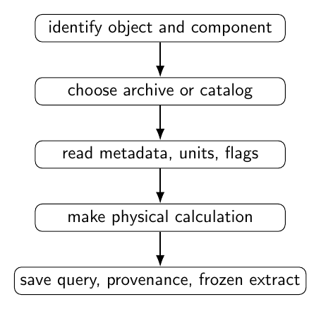
Figure 8. A robust introductory archive workflow separates object identification from catalog
selection, metadata inspection, physical calculation, and reproducible recording of the result.
22 Data provenance is part of the physics
A number without provenance is not yet a trustworthy scientific measurement.
For every value used in an analysis, record when practical:
- database or archive,
- catalog or data release,
- table name,
- source identifier,
- units,
- uncertainty,
- quality flags,
- literature reference,
- retrieval date,
- query or script.
This discipline becomes increasingly important as the series advances from hand calculations to
research-level inference.
23 A first quantitative observing question
Suppose an instrument resolves two stars only when their angular separation exceeds
At
this corresponds to projected separation
At
the same angular resolution corresponds to
The same instrument therefore samples different physical-separation ranges at different
distances.
This simple fact already creates an observational selection function.
24 A first quantitative eclipse question
Consider two solar-radius stars with
If their orbital separation is
then using
we have
| Peclipse | ∼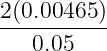 | (36)
|
| ≈ 0.186. | (37) |
So the geometric eclipse probability is of order
A much wider system with the same stellar radii would be much less likely to eclipse.
25 Common mistakes
- Assuming every close pair on the sky is gravitationally bound.
- Treating observational classifications as mutually exclusive physical categories.
- Confusing angular separation with physical separation.
- Forgetting that measured sky separation is projected separation.
- Inserting one instantaneous projected separation into Kepler’s third law as though it
were the orbital semimajor axis.
- Using parallax in milliarcseconds without converting the inversion correctly.
- Assuming the brighter star is always the more massive star.
- Forgetting that spectroscopic masses often contain inclination factors.
- Assuming all binaries eclipse.
- Ignoring observational selection when interpreting a binary sample.
- Treating a SIMBAD value as though it automatically came from a single homogeneous
survey.
- Recording a measurement without its uncertainty, units, source, and data release.
- Confusing a component identifier with the system identifier in a multiple star.
26 Practice exercises
- Explain the difference between a physical binary and an optical double.
- Give one observation that could help establish whether a close angular pair is physically
associated.
- A pair has angular separation 0.8 arcsec at 25 pc. Find the projected separation in
AU.
- A star has parallax 40 MAS. Estimate its distance in pc.
- Explain why projected separation is not generally equal to orbital semimajor axis.
- A binary has a = 6 AU and P = 12 yr. Estimate the total mass in solar masses.
- If a1 = 1 AU and a2 = 3 AU, find M1∕M2.
- An SB2 has K1 = 40 km/s and K2 = 80 km/s. Find M1∕M2.
- Estimate the eclipse probability for R1 + R2 = 0.01 AU and a = 0.10 AU.
- Explain why a close binary can be spectroscopic but not visually resolved.
- Explain why a visually resolved binary need not eclipse.
- Describe why a detached eclipsing SB2 can be especially valuable for stellar
astrophysics.
- List five pieces of provenance that should accompany a catalog measurement.
- Explain why SIMBAD and VizieR are complementary rather than interchangeable.
- Give two examples of observational selection effects in binary star surveys.
27 Summary
Binary stars are physical laboratories because gravity links measurable orbital motion to stellar
properties.
A physical binary is a gravitationally bound pair orbiting a common center of mass.
An optical double is only an apparent close pairing on the sky.
Observed binaries can be visual, astrometric, spectroscopic, eclipsing, or several of these at
once.
The small-angle relation
converts angular scale into projected physical scale.
High-quality parallax measurements provide distance through
A physical orbit and period can provide total mass:
The center of mass provides the mass-ratio relation
Eclipses provide valuable geometric information but are orientation-selected.
The companion BIN01E1 applies these ideas to introductory calculations and live archive
reconnaissance using SIMBAD and VizieR.
BIN02 then develops the observational language needed for quantitative binary star
work: flux, magnitudes, coordinates, time systems, spectra, uncertainties, and FITS
data.
References
References
[1] B. W. Carroll and D. A. Ostlie, An Introduction to Modern Astrophysics, 2nd ed.,
Cambridge University Press, 2017.
[2] R. W. Hilditch, An Introduction to Close Binary Stars, Cambridge University Press,
2001.
[3] G. Torres, J. Andersen, and A. Gimenez, Accurate masses and radii of normal stars:
modern results and applications, Astronomy and Astrophysics Review, 18, 67–126, 2010.
[4] G. Duchene and A. Kraus, Stellar multiplicity, Annual Review of Astronomy and
Astrophysics, 51, 269–310, 2013.
[5] M. Wenger et al., The SIMBAD astronomical database, Astronomy and Astrophysics
Supplement Series, 143, 9–22, 2000.
[6] F. Ochsenbein, P. Bauer, and J. Marcout, The VizieR database of astronomical
catalogues, Astronomy and Astrophysics Supplement Series, 143, 23–32, 2000.