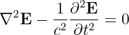
Electromagnetic Waves, Antennas, and RF: Electromagnetic Wave Equation - Exercises and
Complete Worked Solutions
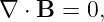
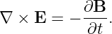
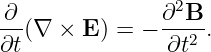
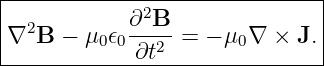
EM16 derived the source-free electromagnetic wave equations from Maxwell’s Equations and then
specialized them to plane waves. This companion article turns those derivations into a sequence of
worked problems. The emphasis is on checking candidate waves rather than merely recognizing
formulas: differentiating traveling profiles, recovering one field from the other, enforcing Maxwell’s
divergence constraints, determining propagation direction, building Standing Waves, extending the
derivation to nonzero sources, and connecting the time-domain wave equation to the
frequency-domain Helmholtz equation.
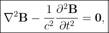
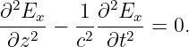
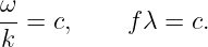
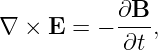
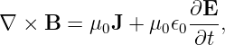
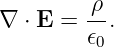
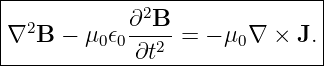
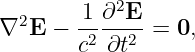
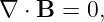
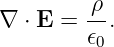
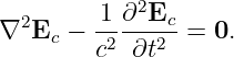
The central vacuum relations are
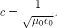
with
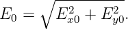
For a monochromatic source-free plane wave,
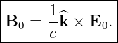
and
These relations should be viewed as consequences of the Maxwell system, not independent
empirical rules [1, 2, 3, 4, 5].
How to use this problem set
Attempt all exercises in Part I before consulting Part II. For each wave problem, use the following
order whenever possible:
- identify the proposed propagation direction from the phase;
- test the wave equation or the relevant Maxwell equation;
- use the divergence equations to check transversality;
- use Faraday and Ampere–Maxwell to determine relative orientation, amplitude, and
phase;
- only then substitute numerical values.
This order helps separate geometry from arithmetic and makes sign errors easier to
detect.
Part I: Exercises
Exercise 1: verify the general traveling profile F(z − ct)
Let
where F is any twice-differentiable function.
Show directly from the chain rule that
Then repeat the argument for
State the propagation direction of each profile and explain why its shape does not change as it
moves.
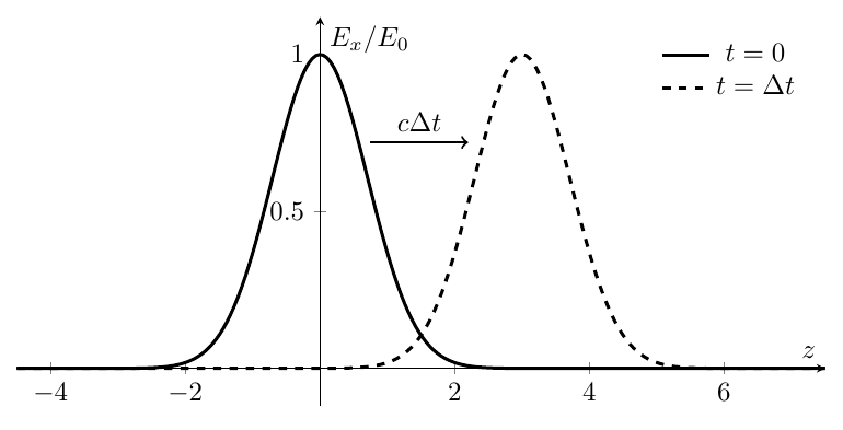
Figure. A profile of the form F(z − ct) is translated a distance cΔt in the +z direction
while retaining the same shape.
Exercise 2: sinusoidal trial solution and the dispersion relation
Consider
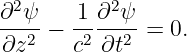
Substitute this field into the one-dimensional wave equation
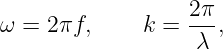
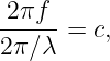
Derive the condition relating ω and k. Then show that
Finally, state the direction of propagation for the phase kz − ωt.
Exercise 3: recover B from a specified electric plane wave
In source-free vacuum let
Assume the corresponding magnetic field has the form
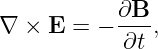
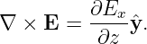
Use Faraday’s law,
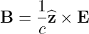
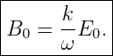
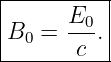
to determine B0 in terms of E0, k, and ω. Then impose the vacuum dispersion relation and show
that
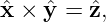
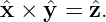
Use the field directions to verify that E × B points in the direction of propagation.
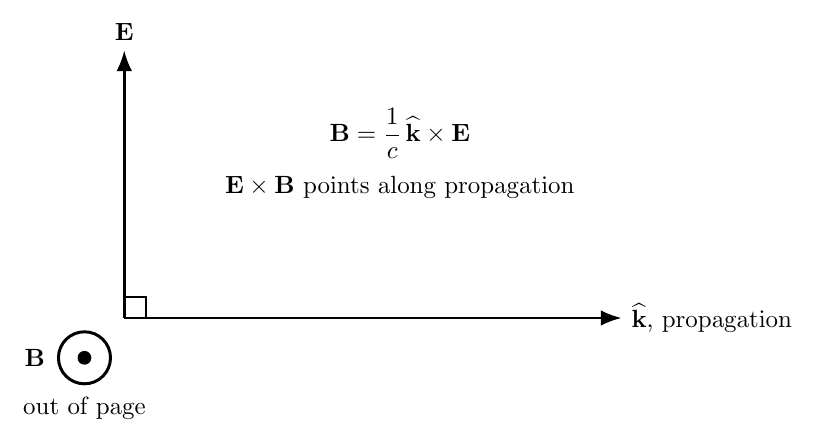
Figure. For a source-free plane wave, E, B, and the propagation direction are mutually
perpendicular, with E × B pointing along propagation.
Exercise 4: radio-frequency wave from magnetic amplitude
A plane electromagnetic wave in vacuum has frequency
and magnetic-field amplitude
The wave propagates in the +z direction and the magnetic field points in the +y direction when
the cosine factor is positive.
Find:
- the wavelength λ;
- the angular frequency ω;
- the Wavenumber k;
- the electric-field amplitude E0;
- the direction of the electric field.
Use c = 299792458 m/s.
Exercise 5: determine propagation direction from field orientation
At a certain phase of a plane wave,
Determine the propagation direction. Then write one possible phase factor for a monochromatic
wave with positive k and positive ω.
Exercise 6: reject a longitudinal candidate using Gauss’s law
Someone proposes the source-free vacuum field
The field satisfies the scalar wave equation if ω = ck.
Compute ∇⋅ E and determine whether the field can nevertheless be a source-free electromagnetic
plane wave. Explain why satisfying the wave equation alone is not enough to guarantee that a field
satisfies the complete Maxwell system.
Exercise 7: full Maxwell consistency with unknown amplitude and phase
Consider
and
Use Faraday’s law and the vacuum Ampere–Maxwell law separately to determine:
- the allowed relative phase δ;
- the amplitude ratio E0∕B0;
- the dispersion relation.
Show that both curl equations are required for the complete result.
Exercise 8: arbitrary linear polarization in the transverse plane
A wave propagates in the +z direction with electric field
Use
to obtain the magnetic field explicitly. Then prove that
and that
where
Exercise 9: build a standing electromagnetic wave from two traveling waves
Two equal-amplitude plane waves propagate in opposite directions:
- Find the corresponding magnetic fields B1 and B2.
- Add the electric fields and simplify using trigonometric identities.
- Add the magnetic fields and simplify.
- Find the positions of the electric-field nodes.
- Find the positions of the magnetic-field nodes.
- Show that an electric node is displaced by λ∕4 from the nearest magnetic node.
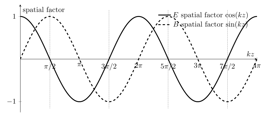
Figure. The spatial factors of the standing-wave electric and magnetic fields are shifted by
one quarter wavelength.
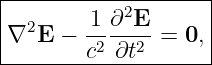
Exercise 10: a Gaussian electromagnetic pulse
Let
- Verify explicitly that Ex satisfies the one-dimensional vacuum wave equation.
- Find the position of the pulse maximum as a function of time.
- Find the magnetic field for a +z-propagating source-free pulse.
- Explain why the pulse is not monochromatic even though every point in the pulse
propagates at the same speed c in vacuum.
Exercise 11: verify the curl–curl identity for a concrete vector field
Consider
Compute both sides of
explicitly and verify that they agree.
This is the identity used in EM16 to turn the two first-order curl equations into second-order wave
equations.
Exercise 12: derive the electric wave equation with sources
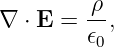
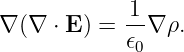
Do not assume ρ = 0 or J = 0. Start from
and
Take one additional curl and derive
Identify the physical source terms on the right-hand side.
Exercise 13: derive the magnetic wave equation with sources
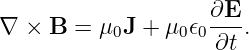
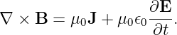
Starting from the general Ampere–Maxwell equation, take its curl and use
and Faraday’s law to derive
Explain why the magnetic source equation contains the curl of current density rather than a
magnetic-charge-density term.
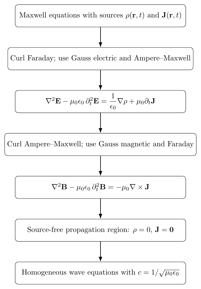
Figure. The homogeneous vacuum wave equations are the source-free limit of more general
wave equations driven by charge and current distributions.
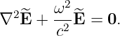
Exercise 14: from the wave equation to the Helmholtz equation
Suppose a source-free electric field is time harmonic and is represented by
Starting from
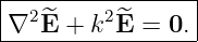
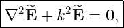
show that the complex spatial amplitude obeys
where
Explain why this conversion is useful in RF, antenna, optics, and steady-state sinusoidal
problems.
Exercise 15: numerical finite-difference check of the wave equation
Let
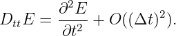
Use centered second differences,
and
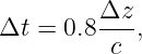
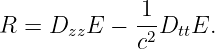
Define the numerical residual
- Write a Julia program that evaluates R at a fixed point.
- Choose Δt = 0.8Δz∕c and refine Δz by factors of two.
- Verify that the normalized residual decreases by approximately a factor of four when
the spacing is halved.
- Explain why that factor is expected for centered second differences.
Part II: Complete Worked Solutions
Solution 1: verify the general traveling profile F(z − ct)
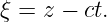
Define
Then
Differentiate with respect to z:
 | = F′(ξ) | (48)
|
| = F′(ξ). | (49) |
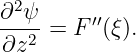
Differentiating once more,
Now differentiate with respect to time:
 | = F′(ξ) | (51)
|
| = −cF′(ξ). | (52) |
Therefore,
 | = −c F′(ξ) F′(ξ) | (53)
|
| = −cF′′(ξ)(−c) | (54)
|
| = c2F′′(ξ). | (55) |
Substitute into the wave equation:
 − −  | = F′′(ξ) − c2F′′(ξ) c2F′′(ξ) | (56)
|
| = 0. | (57) |
Thus every twice-differentiable profile F(z − ct) satisfies the one-dimensional wave equation.
For
the same calculation gives
so G(z + ct) is also a solution.
To identify the direction, hold the profile argument constant. For F(z − ct),
so
As time increases, the same feature moves toward increasing z. Therefore F(z − ct) propagates in
the +z direction.
For G(z + ct),
so the profile propagates in the −z direction.
The shape is preserved because the function itself is not changing; only its argument is translated
in space.
Solution 2: sinusoidal trial solution and the dispersion relation
Start with
The second spatial derivative is
The second time derivative is
Substitute into the wave equation:
− k2E
0 cos(kz − ωt) − ![[ 2 ]
− ω E0cos(kz − ωt)](https://images.physicslibrary.org/cache/objects/1240/make4ht/ElectromagneticWavesElectromagneticWaveEquationExercisesAndCompleteWorkedSolutions67x.png) | = 0. | (66) |
For a nontrivial wave,
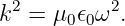
Therefore,
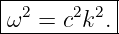
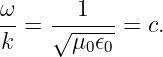
For positive frequency and positive wavenumber,
Hence the phase velocity is
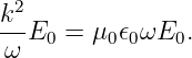
Using
we obtain
so
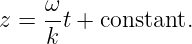
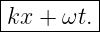
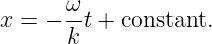
Finally, a surface of constant phase satisfies
which gives
Thus kz − ωt describes propagation in the +z direction.
Solution 3: recover B from a specified electric plane wave
The electric field is
Because only Ex is nonzero and it depends only on z,
Since
we have
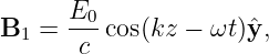
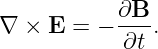
The proposed magnetic field is
Its time derivative is
Faraday’s law requires
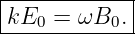
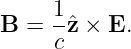
Therefore,
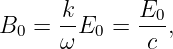
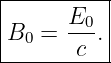
For a vacuum wave,
so
The cross product is
Thus the field orientation is consistent with propagation in the +z direction.
Solution 4: radio-frequency wave from magnetic amplitude
The frequency is
The wavelength is
| λ | =  | (88)
|
| = 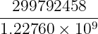 m m | (89)
|
| ≈ 0.244210 m. | (90) |
Therefore,
The angular frequency is
| ω | = 2πf | (92)
|
| = 2π(1.22760 × 10⁹) | (93)
|
| ≈ 7.71324 × 10⁹ rad/s. | (94) |
Thus,
The wavenumber is
| k | =  | (96)
|
| ≈ 25.7286 rad/m. | (97) |
Therefore,
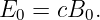
For a vacuum plane wave,
With
we obtain
| E0 | = (299792458)(2.50 × 10⁻⁹) | (101)
|
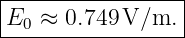
| ≈ 0.74948 V/m. | (102) |
Hence,
The wave travels in +z and B points in +y. We need
Since
the electric field points in the +x direction when the cosine factor is positive.
Solution 5: determine propagation direction from field orientation
For a source-free plane wave, the propagation direction follows the direction of
Here
Therefore,
| E × B | ∥y × (−z) | (108)
|
| = −x. | (109) |
Thus the wave propagates in the negative x direction:
A convenient phase for propagation in the −x direction is
Indeed, holding phase constant gives
or
The constant-phase surface therefore moves toward decreasing x.
Solution 6: reject a longitudinal candidate using Gauss’s law
The proposed field is
Its divergence is
| ∇⋅ E | =  | (115)
|
| = −kE0 sin(kz − ωt). | (116) |
This is generally nonzero. But in source-free vacuum, Gauss’s Law requires
Therefore the proposed longitudinal field is not an allowed source-free electromagnetic plane
wave.
The important lesson is that the second-order wave equation is a consequence of Maxwell’s
equations, but by itself it does not encode every Maxwell constraint. A candidate field can
satisfy
while failing
Therefore a complete electromagnetic solution must satisfy both the wave equation and the
relevant Maxwell constraints.
Solution 7: full Maxwell consistency with unknown amplitude and phase
Let
Then
and
Faraday’s law gives
Meanwhile,
Thus
for every z and t. The simplest nontrivial possibility is that the fields are in phase,
with
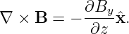
Now apply Ampere–Maxwell. Since only By depends on z,
For δ = 0,
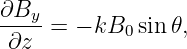
so
The right-hand side is
μ0𝜖0 | = μ0𝜖0ωE0 sin 𝜃x. | (131) |
Therefore,
Use the Faraday result
Substitution gives
Cancel E0 and multiply by ω:
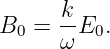
Hence,
Thus
Finally,
or
Faraday’s law determines the relative amplitude and phase relation once ω∕k is known.
Ampere–Maxwell supplies the second relation needed to determine the vacuum dispersion relation
itself.
Solution 8: arbitrary linear polarization in the transverse plane
The electric field is
For propagation in +z,
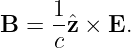
Use
Therefore,
| B | =   cos(kz − ωt). cos(kz − ωt). | (143) |
Thus
Now take the dot product of the amplitude vectors:
| E0 ⋅ B0 | =  ⋅ ⋅  | (145)
|
| =   | (146)
|
| = 0. | (147) |
Therefore,
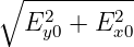
The magnetic amplitude is
Hence,
This result does not depend on which transverse direction the linear polarization chooses.
Solution 9: build a standing electromagnetic wave from two traveling waves
For the +z wave,
The associated magnetic field is
because
For the −z wave,
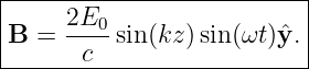
Now E2 × B2 must point in −z, so the magnetic field reverses direction:
Add the electric fields:
| E | = E0![[cos(kz − ωt) + cos(kz + ωt)]](https://images.physicslibrary.org/cache/objects/1240/make4ht/ElectromagneticWavesElectromagneticWaveEquationExercisesAndCompleteWorkedSolutions152x.png) x. x. | (157) |
Using
we obtain
Now add the magnetic fields:
| B | =  ![[cos(kz − ωt) − cos(kz + ωt)]](https://images.physicslibrary.org/cache/objects/1240/make4ht/ElectromagneticWavesElectromagneticWaveEquationExercisesAndCompleteWorkedSolutions156x.png) y. y. | (160) |
Using
we obtain
Electric nodes occur where
Thus
or
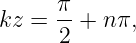
Magnetic nodes occur where
so
and therefore
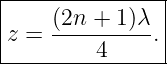
The nearest electric and magnetic nodes differ by
This spatial offset is a characteristic feature of a standing electromagnetic wave.
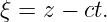
Solution 10: a Gaussian electromagnetic pulse
Define
Then
This is exactly the form F(z − ct) from Exercise 1, so it must satisfy the one-dimensional wave
equation. We can also verify it directly.
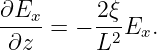
First,
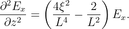
Differentiating again,
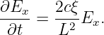
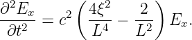
For the time derivative,
Differentiating again gives
Therefore,
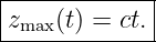
The pulse maximum occurs when the exponent is zero:
Thus
For a +z-propagating pulse with E ∥x,
Hence
The Gaussian pulse is not monochromatic because it is localized in space. A localized waveform
requires a superposition of many wavenumbers and therefore many frequencies. In nondispersive
vacuum, all of those spectral components satisfy ω = ck and therefore propagate with the same
speed c, so the pulse retains its shape.
Solution 11: verify the curl–curl identity for a concrete vector field
The vector field is
First compute its curl:
| ∇× A | = 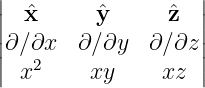 | (182)
|
| = 0x − zy + yz. | (183) |
Now curl that result:
| ∇× (∇× A) | = ∇× | (184)
|
| = 2x. | (185) |
So the left-hand side is
Now compute the right-hand side. The divergence is
| ∇⋅ A | =  + +  + +  | (187)
|
| = 2x + x + x | (188)
|
| = 4x. | (189) |
Therefore,
The vector Laplacian is obtained component by component:
Thus
Hence
| ∇(∇⋅ A) −∇2A | = 4x − 2x | (193)
|
| = 2x. | (194) |
Therefore,
The identity is verified for this explicit field.
Solution 12: derive the electric wave equation with sources
Begin with Faraday’s law:
Take the curl of both sides:
Use the curl–curl identity:
Gauss’s law gives
so
Ampere–Maxwell gives
Therefore,
− (∇× B) (∇× B) | = −μ0 − μ0𝜖0 − μ0𝜖0 . . | (202) |
Substitute both results:
Rearrange:
The source terms are therefore:
- the spatial gradient of charge density, (1∕𝜖0)∇ρ;
- the time variation of current density, μ0∂J∕∂t.
When both vanish in the local propagation region, the equation reduces to the homogeneous
vacuum wave equation derived in EM16.
Solution 13: derive the magnetic wave equation with sources
Start from Ampere–Maxwell:
Take the curl:
Use the curl–curl identity:
Gauss’s law for magnetism gives
so the left side becomes
Faraday’s law gives
Therefore,
Substitute:
Multiply by −1 and rearrange:
There is no term proportional to a magnetic charge density because Maxwell’s classical theory
contains
rather than a magnetic analogue of
Thus magnetic-wave source structure enters through circulating electric current, represented by
∇× J.
Solution 14: from the wave equation to the Helmholtz equation
Represent the real physical field as
Because the wave equation is linear, it is sufficient to work with the complex field
The Laplacian acts only on the spatial amplitude:
The second time derivative is
 | = (−iω)2Ee−iωt | (219)
|
| = −ω2Ee−iωt. | (220) |
Substitute into
This gives
Since the exponential factor is never zero,
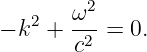
Define
Then
This is the vector Helmholtz equation in a homogeneous source-free region.
The time-domain wave equation describes general transients and arbitrary time dependence. The
Helmholtz equation removes the known sinusoidal time dependence and leaves a purely spatial
boundary-value problem. That makes it especially useful for steady-state RF fields, antennas,
resonators, diffraction, and monochromatic optics.
Solution 15: numerical finite-difference check of the wave equation
A direct Julia implementation is:
using Printf

c = 299_792_458.0
lambda = 1.0
k = 2pi / lambda
omega = c * k
E0 = 1.0

E(z, t) = E0 * cos(k*z - omega*t + 0.37)

z0 = 0.23
t0 = 0.17 / c

println(" N normalized residual")

for N in (40, 80, 160, 320)
dz = lambda / N
dt = 0.8 * dz / c

dzz = (E(z0 + dz, t0) - 2E(z0, t0) + E(z0 - dz, t0)) / dz^2
dtt = (E(z0, t0 + dt) - 2E(z0, t0) + E(z0, t0 - dt)) / dt^2

R = dzz - dtt / c^2
Rnorm = abs(R) / (k^2 * abs(E(z0, t0)))

@printf("%4d %.6e\n", N, Rnorm)
end
The centered second-difference formulas are second-order accurate:
and
With
both truncation errors scale as (Δz)2.
For the test point and phase used above, representative normalized residuals are approximately
for N = 40, 80, 160, 320, respectively.
Each time N doubles, Δz is halved. A second-order error should therefore change by
approximately
That is exactly the trend in the numerical residual. The finite-difference experiment
therefore checks two things at once: the analytic plane wave satisfies the continuum wave
equation, and the chosen numerical approximation converges at the expected second-order
rate.
1 What EM16E1 adds to the series
EM16 derived the electromagnetic wave equation and its basic plane-wave consequences. EM16E1
turns those results into working tools.
The main progression is
The most important conceptual point is that the scalar-looking wave equation is necessary but not
sufficient for a physical electromagnetic field. The complete field must also satisfy the Maxwell
divergence and curl equations, which enforce transversality, field orientation, phase relationships,
and the amplitude relation E0 = cB0.
A natural next topic is electromagnetic energy and power flow: electric and magnetic energy
density, the Poynting vector, intensity, and inverse-square spreading.
References
[1] David J. Griffiths, Introduction to Electrodynamics, 4th ed., Cambridge University
Press, 2017.
[2] Edward M. Purcell and David J. Morin, Electricity and Magnetism, 3rd ed.,
Cambridge University Press, 2013.
[3] Samuel J. Ling, Jeff Sanny, and William Moebs, University Physics, Volume 2,
OpenStax, 2016, sections on Maxwell’s equations and electromagnetic waves.
[4] Richard P. Feynman, Robert B. Leighton, and Matthew Sands, The Feynman Lectures
on Physics, Volume II, Addison-Wesley, 1964, chapters on electromagnetic waves and
Maxwell’s equations.
[5] Massachusetts Institute of Technology, 8.02 Physics II: Electricity and Magnetism,
MIT OpenCourseWare, materials on Maxwell’s equations and electromagnetic waves.
[6] James Clerk Maxwell, “A Dynamical Theory of the Electromagnetic Field,”
Philosophical Transactions of the Royal Society of London, vol. 155, pp. 459–512, 1865.

![[parent]](https://images.physicslibrary.org/images/uparrow.png)


















![[ (z − ct)2]
Ex (z,t) = E0 exp − -----2--- .
L](https://images.physicslibrary.org/cache/objects/1240/make4ht/ElectromagneticWavesElectromagneticWaveEquationExercisesAndCompleteWorkedSolutions28x.png)










































































![|--------------------------------|
| E [ (z − ct)2] |
|B(z,t) = --0exp − -----2--- ˆy.|
-----------c-----------L----------](https://images.physicslibrary.org/cache/objects/1240/make4ht/ElectromagneticWavesElectromagneticWaveEquationExercisesAndCompleteWorkedSolutions178x.png)

















![[ ]
−iωt 2^ ω2-^
e ∇ E + c2 E = 0.](https://images.physicslibrary.org/cache/objects/1240/make4ht/ElectromagneticWavesElectromagneticWaveEquationExercisesAndCompleteWorkedSolutions217x.png)