Electromagnetic Waves, Antennas, and RF: Deriving the Electromagnetic Wave Equation from
Maxwell’s Equations
EM15 assembled Maxwell’s Equations into one coupled field theory. The next question is the
central one for electromagnetic-wave physics:
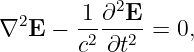
The answer is yes. In a source-free vacuum, the two curl equations combine into second-order
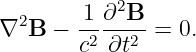
partial differential equations for both the electric field E and magnetic field B. Those equations
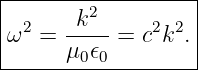
have exactly the mathematical form of wave equations, and their propagation speed
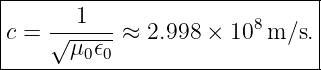
is
This article derives that result carefully and then specializes it to a one-dimensional sinusoidal
plane wave. Along the way we will see why electromagnetic waves are transverse, why E and B are
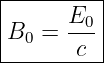
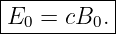
perpendicular to each other, why they oscillate in phase in vacuum, and why their amplitudes
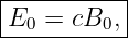
satisfy E0 = cB0 [1, 2, 3, 4, 5].
1 Start from the source-free Maxwell system
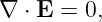
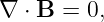
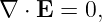
In a region containing no free charge and no conduction current,
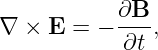
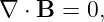
The four differential Maxwell equations reduce to
and
The first two equations are divergence constraints. The last two are dynamical curl equations. The
wave equations emerge when the two curl equations are combined.
2 The strategy: take one more curl
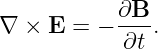
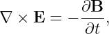
Faraday’s law already couples spatial variation of E to time variation of B:
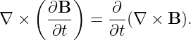
To obtain an equation involving E alone, take the curl of both sides:
Assuming the fields are sufficiently smooth, spatial and temporal differentiation commute,
so
Therefore,
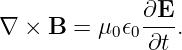
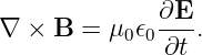
Now Ampere–Maxwell can eliminate B from the right-hand side.
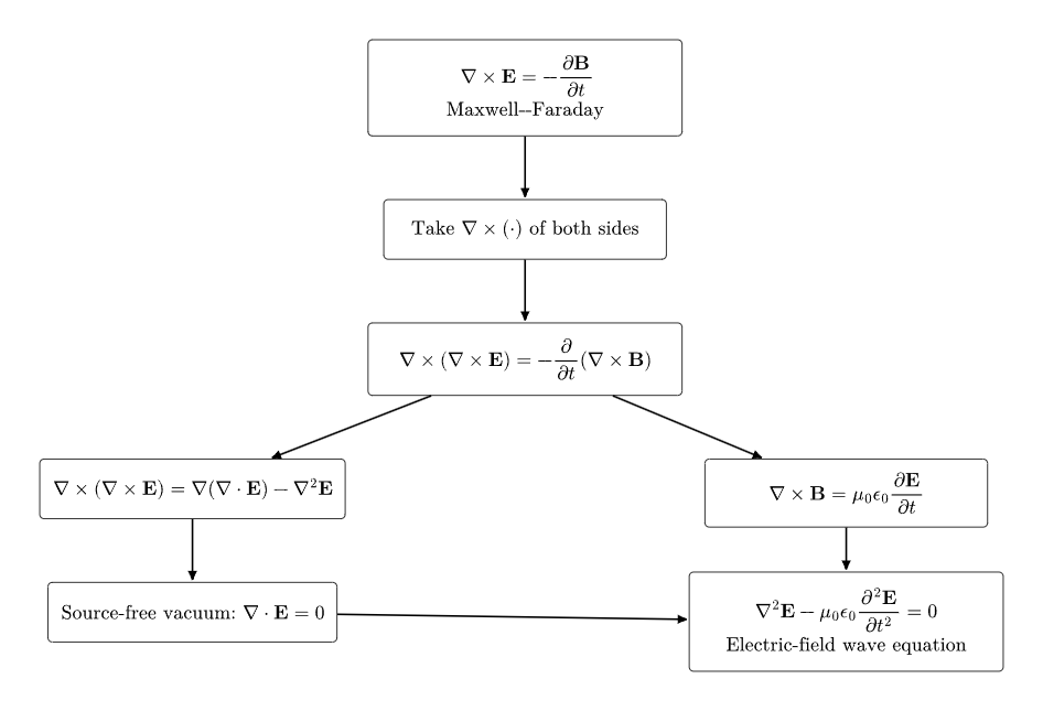
Figure. The electric-field wave equation is obtained by taking the curl of Faraday’s law,
using the curl–curl identity, imposing the vacuum divergence constraint, and substituting
the vacuum Ampere–Maxwell equation.
3 The curl–curl vector identity
The key vector-calculus identity is
Here ∇2A means the vector Laplacian applied component by component in Cartesian
coordinates:
Apply the identity to E:
In source-free vacuum,
so
Hence,
This is the step where Gauss’s Law for electricity enters the wave-equation derivation.
4 Derivation of the electric-field wave equation
Return to
Use the vacuum Ampere–Maxwell law,
Then
− (∇× B) (∇× B) | = − 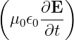 | (20)
|
| = −μ0𝜖0 . . | (21) |
Using the result from the previous section,
Cancel the minus signs:
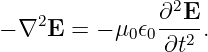
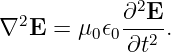
Equivalently,
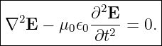
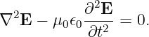
This is the electromagnetic wave equation for the electric field in source-free vacuum.
5 Derivation of the magnetic-field wave equation
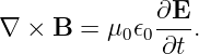
The same reasoning can be repeated starting from the vacuum Ampere–Maxwell law:
Take the curl:
Use Faraday’s law,
so
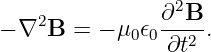
The curl–curl identity gives
Since
we obtain
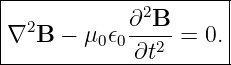
Therefore,
Thus both fields obey the same propagation equation.
6 Comparison with the generic wave equation
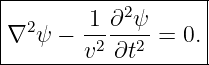
A scalar wave field ψ(r,t) propagating at speed v satisfies
Compare this with the electric-field equation
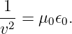
The coefficients must correspond:
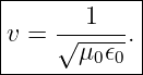
Therefore,
For electromagnetic fields in vacuum this speed is denoted by c:
Maxwell’s field equations therefore predict propagating waves whose speed is the speed of light.
Historically, the agreement between the electromagnetic speed scale and measured optical
propagation speed was one of the decisive clues that light is an electromagnetic phenomenon
[6, 4].
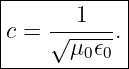
7 Dimensional check of the speed
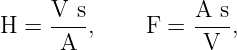
It is worth checking the units. Using
and
we have
| [μ0𝜖0] | =  . . | (40) |
Since
then
Therefore,
and
as required for a speed.
8 What source-free vacuum really means
The condition
inside the region of interest does not mean that no source exists anywhere in the universe. An
antenna can create a disturbance near its Conductors, and after that disturbance leaves the source
region it can propagate through a region where
The vacuum wave equation describes that propagation region.
This distinction is essential in radio physics: sources launch the wave, but the wave does not need
local charges and currents at every point along its later path.
9 One-dimensional reduction
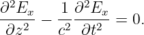
Suppose the fields vary only with position z and time t. For one Cartesian component, the
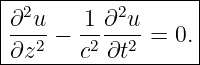
three-dimensional wave equation reduces to
Here u can represent a Cartesian component such as Ex or By.
The standard traveling-wave solutions are
The first term moves in the +z direction at speed c. The second moves in the −z direction at
speed c.
10 Why F(z − ct) moves without changing shape
Consider
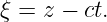
Define
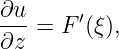
Then
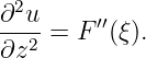
and
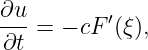
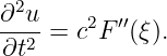
For the time derivatives,
so
Substituting into the one-dimensional wave equation gives
 − −  | = F′′(ξ) − c2F′′(ξ) c2F′′(ξ) | (55)
|
| = 0. | (56) |
Therefore any sufficiently smooth waveform F can propagate rigidly at speed c.
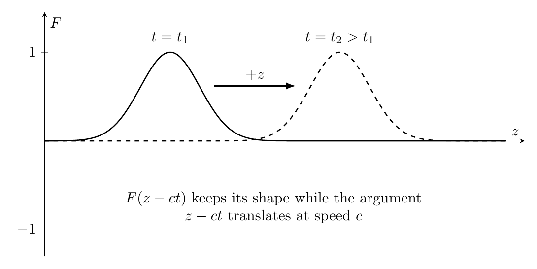
Figure. A function of z − ct translates in the +z direction at speed c without changing its
mathematical shape.
11 Sinusoidal solution and the dispersion relation
Now consider a monochromatic electric field of the form
The second spatial derivative is
The second time derivative is
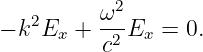
Insert these into
Then
For a nonzero field,
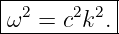
For a wave traveling in the +z direction we take positive ω and k, giving
Thus the phase velocity is
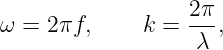
Using
we recover
12 Worked example: GPS L1 wavelength in vacuum
The GPS L1 carrier frequency is
Using
we obtain
| λL1 | = 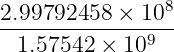 m m | (69)
|
| ≈ 0.1903 m. | (70) |
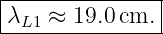
Therefore,
The wave equation therefore connects the field theory of Maxwell directly to the wavelength scales
encountered in RF and GNSS engineering.
13 Recovering the magnetic field from Faraday’s law
Consider an electromagnetic wave traveling in the +z direction with
Assume the magnetic field has the form
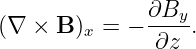
For this electric field,
Since
Faraday’s law gives
But
Therefore,
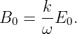
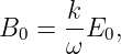
So
Using ω∕k = c,
or equivalently
This relation is specific to plane electromagnetic waves in vacuum.
14 The electric and magnetic fields are in phase
The electric and magnetic fields just derived are
and
Both contain the same phase
Therefore their maxima, minima, and zero crossings occur at the same positions and
times.
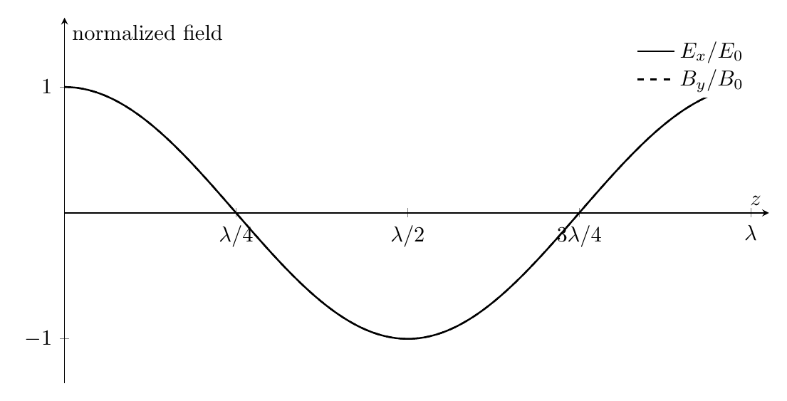
Figure. For a vacuum plane wave, normalized Ex and By have the same phase
dependence. The plotted curves coincide; the dashed curve is shown only to identify the
magnetic field separately.
15 Why a plane electromagnetic wave is transverse
Let a monochromatic plane electric field be written in the general form
Take its divergence:
In source-free vacuum,
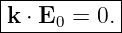
for all positions and times. Therefore,
Hence
Applying the same argument to
gives
Both fields are therefore transverse to the propagation direction.
16 Why E, B, and k form an orthogonal triad
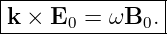
For a plane wave, Faraday’s law gives the vector amplitude relation
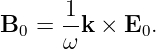
Therefore,
Since
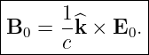
we can write
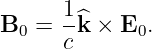
This immediately shows that B0 is perpendicular to both k and E0.
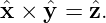
For a wave traveling in the +z direction,
and
Thus the propagation direction agrees with
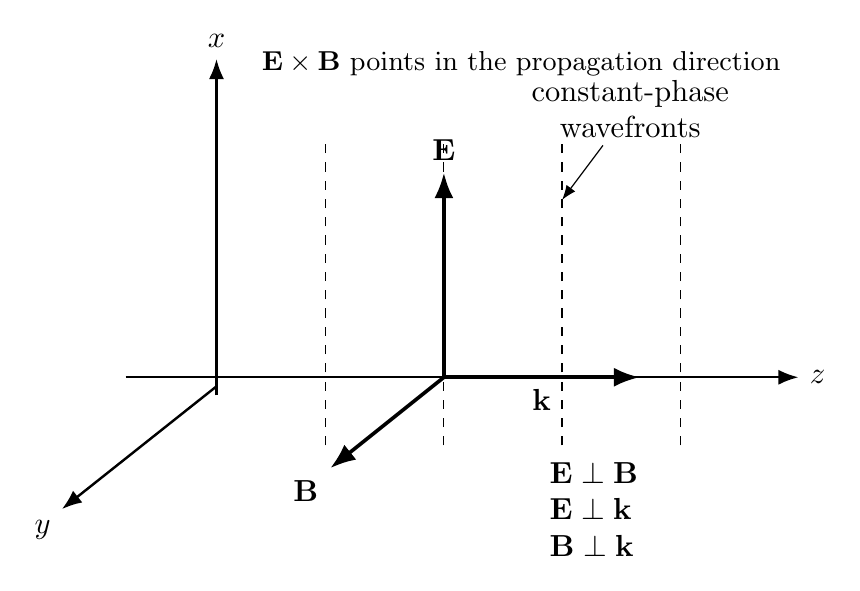
Figure. A vacuum plane wave is transverse: E, B, and the propagation vector k are
mutually perpendicular, and E × B points in the propagation direction.
17 Checking the same plane wave with Ampere–Maxwell
For
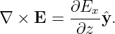
the x component of the curl is
Since
we obtain
Meanwhile,
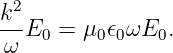
Ampere–Maxwell requires
Using
we obtain
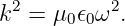
For E0≠0,
Therefore,
The two curl equations are therefore mutually consistent with the same propagation speed and
amplitude relation.
18 A useful hierarchy of equations
The derivation can now be organized into four levels.
At the field-law level:
At the wave-equation level:
At the monochromatic plane-wave level:
And the geometry and dispersion relations are
These are not separate assumptions. They are progressively specialized consequences of Maxwell’s
equations.
19 Common mistakes
- Forgetting that the wave-equation derivation shown here assumes a source-free region,
so ρ = 0 and J = 0.
- Taking the curl of Faraday’s law but forgetting that the right-hand side becomes a
time derivative of ∇× B.
- Using ∇× (∇× E) = −∇2E without first invoking ∇⋅ E = 0.
- Dropping a minus sign in the curl–curl identity.
- Confusing the scalar Laplacian ∇2 with the divergence or curl operators.
- Assuming that source-free means the wave has never been created by a source; it means
only that the local propagation region contains no charge or conduction-current source
terms.
- Writing E0 = B0. In SI units their numerical amplitudes differ by the factor c:
E0 = cB0.
- Assuming every possible electromagnetic field configuration is transverse. The
transverse relations derived here are for source-free plane waves.
- Treating k as a frequency. The angular frequency is ω; the Wavenumber k = 2π∕λ
measures spatial phase variation.
- Forgetting that F(z − ct) moves in the +z direction, while G(z + ct) moves in the −z
direction.
20 What EM16 adds to the series
EM15 showed that Maxwell’s equations form a self-consistent coupled system. EM16 now shows
that the same system contains wave propagation intrinsically.
The central chain is
For a monochromatic plane wave, Maxwell’s equations further imply
and
The next natural step is to study electromagnetic-wave energy flow: energy density, the Poynting
vector, intensity, and how power spreads through space.
References
[1] David J. Griffiths, Introduction to Electrodynamics, 4th ed., Cambridge University
Press, 2017.
[2] Edward M. Purcell and David J. Morin, Electricity and Magnetism, 3rd ed.,
Cambridge University Press, 2013.
[3] Samuel J. Ling, Jeff Sanny, and William Moebs, University Physics, Volume 2,
OpenStax, 2016, sections on Maxwell’s equations and electromagnetic waves.
[4] Richard P. Feynman, Robert B. Leighton, and Matthew Sands, The Feynman Lectures
on Physics, Volume II, Addison-Wesley, 1964, chapters on electromagnetic waves and
Maxwell’s equations.
[5] Massachusetts Institute of Technology, 8.02 Physics II: Electricity and Magnetism,
MIT OpenCourseWare, materials on Maxwell’s equations and electromagnetic waves.
[6] James Clerk Maxwell, “A Dynamical Theory of the Electromagnetic Field,”
Philosophical Transactions of the Royal Society of London, vol. 155, pp. 459–512, 1865.














![[μ0] = H/m](https://images.physicslibrary.org/cache/objects/1239/make4ht/ElectromagneticWavesDerivingTheElectromagneticWaveEquationFromMaxwellsEquations39x.png)
![[𝜖0] = F/m,](https://images.physicslibrary.org/cache/objects/1239/make4ht/ElectromagneticWavesDerivingTheElectromagneticWaveEquationFromMaxwellsEquations40x.png)

![-s2-
[μ0𝜖0] = m2 ,](https://images.physicslibrary.org/cache/objects/1239/make4ht/ElectromagneticWavesDerivingTheElectromagneticWaveEquationFromMaxwellsEquations44x.png)
![[ ]
√-1---- = m-,
μ0𝜖0 s](https://images.physicslibrary.org/cache/objects/1239/make4ht/ElectromagneticWavesDerivingTheElectromagneticWaveEquationFromMaxwellsEquations45x.png)