Electromagnetic Waves, Antennas, and RF: The Laplacian and the 3D Wave Equation - Exercises and Complete Worked Solutions

This companion article provides self-study exercises for EM04, The Laplacian and the 3D wave equation. All exercises are stated first. Complete worked solutions follow in Part II.

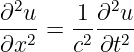
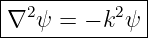
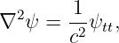
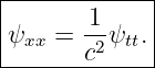
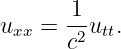
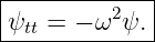
The exercises reinforce the central bridge from the one-dimensional wave equation

∂2u 1 ∂2u ∂x2- = c2 ∂t2-

(1)

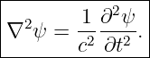
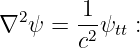
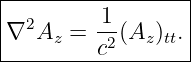
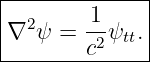
to the three-dimensional equation

|--------------| | 2 1 ∂2ψ | ∇ ψ = -2---2 . --------c--∂t---

(2)

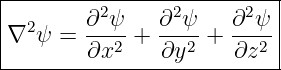
The Laplacian in Cartesian Coordinates is

|--------------------------| | 2 ∂2-ψ ∂2-ψ ∂2-ψ | |∇ ψ = ∂x2 + ∂y2 + ∂z2 | ---------------------------

(3)

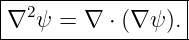
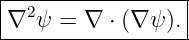
and can also be written

|-2---------------| ∇--ψ-=--∇-⋅ (∇-ψ).-

(4)

For the plane wave

ψ (r,t) = A cos(k ⋅ r − ωt + ϕ0),

(5)

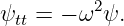
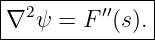
EM04 showed that

|-2--------2--| ∇--ψ-=--− k-ψ--

(6)

and

|------------| |ψtt = − ω2ψ.| --------------

(7)

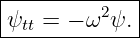
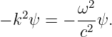
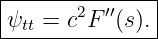
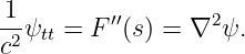
Therefore a nondispersive wave satisfying the three-dimensional wave equation must obey

|--------| -ω-=-ck,-|

(8)

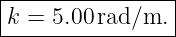
with

k = 2π-, ω = 2πf, c = fλ. λ

(9)

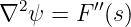
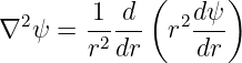
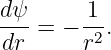
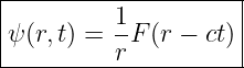
For an outgoing spherically spreading wave in three dimensions,

|--------------------------------| | 1 | |ψ (r,t) = --F(r − ct), r > 0. | ----------r----------------------

(10)

These results follow the notation and scope of EM04 [3, 2, 6, 7].

How to use this problem set

Attempt all exercises in Part I before reading Part II. In each problem, first identify the spatial operator and the dimensionality of the field. Then check the result against the structure of the wave equation. For plane-wave problems, keep the scalar Wavenumber k = |k| distinct from the vector k.

Part I: Exercises

Exercise 1: compute a Cartesian Laplacian

Let

ψ (x,y,z) = x2 + 2y2 − 3z2 + 4xy.

(11)

Compute ∇²ψ.

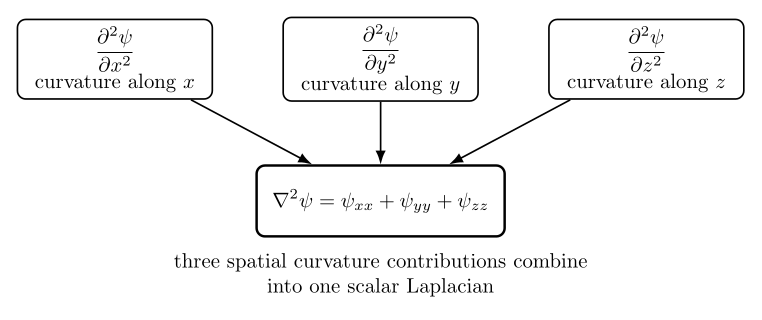
Figure. The Cartesian Laplacian adds the second-derivative contributions from the three spatial directions.

Exercise 2: recover the Laplacian as divergence of the gradient

For

ϕ(x,y,z ) = x2y + yz2,

(12)

find:

∇ϕ;
∇⋅ (∇ϕ);
∇²ϕ directly from second derivatives.

Verify that the answers in parts (b) and (c) agree.

Exercise 3: Laplace’s equation

Determine whether each scalar field satisfies Laplace’s equation

∇2 ψ = 0.

(13)

ψ₁ = x² − y²;
ψ₂ = x² + y² + z²;
ψ₃ = xy + yz + zx.

Exercise 4: reduction from 3D to 1D

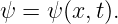
Suppose a field depends only on x and t:

ψ = ψ (x,t).

(14)

Starting from

∇2 ψ = 1-ψtt, c2

(15)

show explicitly that the equation reduces to

|------------| | 1 | |ψxx = -2ψtt.| -------c------

(16)

Exercise 5: verify a plane-wave solution

Let

ψ(r,t) = A cos(k ⋅ r − ωt).

(17)

Show that

∇2 ψ = − k2ψ

(18)

and

ψ = − ω2ψ. tt

(19)

Then substitute into the three-dimensional wave equation and derive the required dispersion relation.

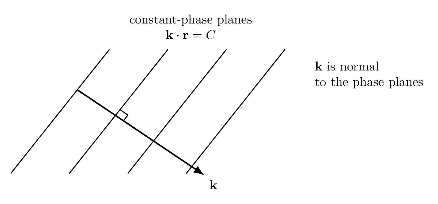
Figure. The wave vector k is normal to constant-phase planes. Its magnitude k enters the plane-wave dispersion relation.

Exercise 6: wave vector, wavelength, and frequency

A plane wave propagates with

k = (3ˆx + 4ˆy) rad/m

(20)

in a medium where

8 c = 2.00 × 10 m/s.

(21)

Find:

k = |k|;
the wavelength λ;
the angular frequency ω;
the ordinary frequency f;
the unit propagation direction k.

Exercise 7: wavelength of a GPS-frequency radio wave

Treat a radio wave in vacuum as propagating at

c = 299792458 m/s.

(22)

For the GPS L1 carrier frequency

9 f = 1.57542 × 10 Hz,

(23)

find:

the wavelength λ;
the scalar wavenumber k.

This problem uses the wave-equation relation c = fλ only; detailed electromagnetic physics is reserved for later entries.

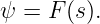
Exercise 8: arbitrary traveling profile in three dimensions

Let

ψ (r,t) = F (s), s = ˆn ⋅ r − ct,

(24)

where n is a constant unit vector.

Using the chain rule, show that

∇2 ψ = F′′(s)

(25)

and

ψtt = c2F ′′(s).

(26)

Conclude that any sufficiently smooth profile F of this form satisfies the 3D wave equation.

Exercise 9: the radial Laplacian

For a spherically symmetric scalar field

ψ = ψ (r),

(27)

use the radial Laplacian

( ) 2 1 d 2dψ ∇ ψ = r2dr- r dr-

(28)

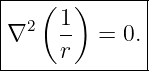
to compute ∇²(1∕r) for r > 0.

Exercise 10: spherical-wave amplitude spreading

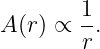
An outgoing spherical wave has amplitude proportional to 1∕r. At radius r₁, the amplitude is A₁. At radius

r2 = 4r1,

(29)

find:

A₂∕A₁;
the corresponding ratio of a quantity proportional to amplitude squared.

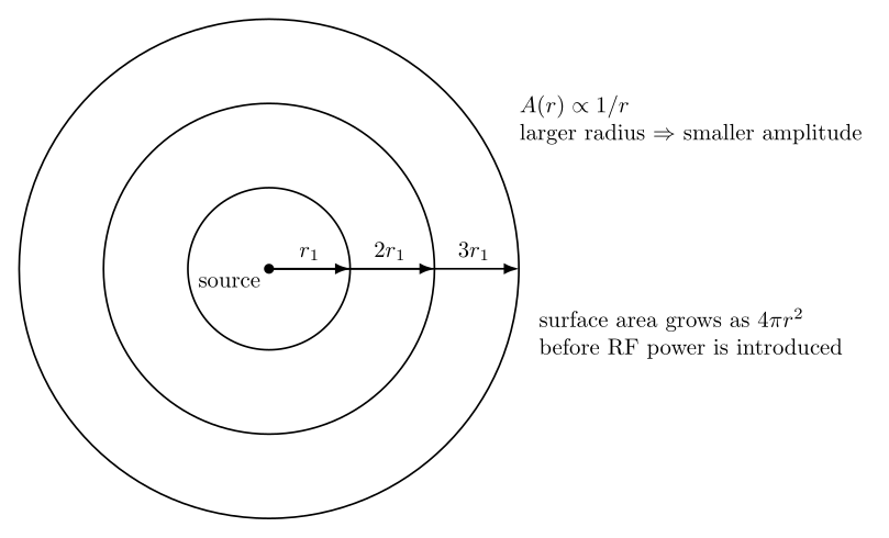
Figure. A spherical disturbance spreads over larger spherical surfaces as radius increases. The wave amplitude scales as 1∕r in the ideal outgoing solution.

Exercise 11: reduce a spherical wave to a 1D radial equation

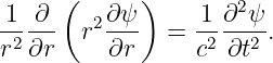
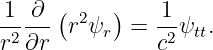
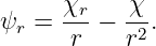
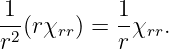
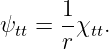
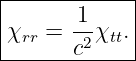
For a spherically symmetric wave ψ(r,t), the wave equation is

( ) 2 1--∂- r2∂ψ- = 1-∂-ψ-. r2∂r ∂r c2 ∂t2

(30)

Define

χ (r,t) = rψ (r,t).

(31)

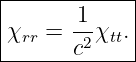
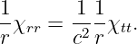
Show that for r > 0 the equation becomes

|------------| | 1 | |χrr = c2χtt.| -------------

(32)

Exercise 12: vector wave equation component by component

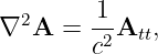
Suppose a vector field is

A (r,t) = Ax(r,t)ˆx + Ay (r,t)ˆy + Az (r,t)zˆ.

(33)

1 ∇2A = -2Att, c

(34)

write the three scalar component equations explicitly.

Then verify that

A = A0yˆcos(kz − ωt)

(35)

satisfies the vector wave equation when ω = ck.

Exercise 13: identify which functions satisfy the 1D wave equation

For each candidate below, determine whether it satisfies

uxx = -1utt. c2

(36)

Assume all constants are nonzero unless stated otherwise.

u₁ = A cos(kx − ckt);
u₂ = A cos(kx − 2ckt);
u₃ = F(x − ct) for a twice-differentiable F;
u₄ = x² + c²t².

Exercise 14: synthesis - geometry, phase, wavelength, and frequency

A plane wave is

ψ(r,t) = A cos(k ⋅ r − ωt + ϕ0)

(37)

with

k = (4ˆx − 3 ˆy)rad/m, c = 3.00 × 108m/s, ϕ0 = π-. 4

(38)

Find:

k;
k;
λ;
ω;
f;
the phase at r = (1, 2, 0) m and t = 2.0 ns.

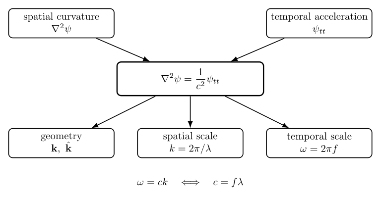
Figure. The 3D wave equation links spatial curvature, temporal acceleration, propagation geometry, wavelength, and frequency.

Part II: Complete Worked Solutions

Solution 1: compute a Cartesian Laplacian

Given

2 2 2 ψ = x + 2y − 3z + 4xy,

(39)

we compute the second derivatives one coordinate at a time:

∂2ψ ∂2 ψ ∂2ψ --2-= 2, ---2 = 4, ---2 = − 6. ∂x ∂y ∂z

(40)

The mixed term 4xy contributes nothing to any pure second derivative. Therefore,

∇2 ψ = 2 + 4 − 6 = 0.

(41)

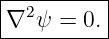
Hence

|----------| |∇2 ψ = 0. | -----------

(42)

This field is harmonic: it satisfies Laplace’s equation.

Solution 2: recover the Laplacian as divergence of the gradient

The scalar field is

2 2 ϕ = x y + yz .

(43)

Its gradient is

∇ϕ	= x + y + z	(44)
	= 2xyx + (x² + z²)y + 2yzz.	(45)

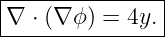
Thus

|--------------------------------| |∇ ϕ = 2xyxˆ+ (x2 + z2)ˆy + 2yz ˆz.| ----------------------------------

(46)

Now take the divergence:

∇⋅ (∇ϕ)	= + +	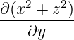(47)
	= 2y + 0 + 2y	(48)
	= 4y.	(49)

Therefore,

|--------------| ∇--⋅ (∇-ϕ)-=-4y.

(50)

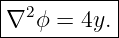
Directly,

ϕ = 2y, ϕ = 0, ϕ = 2y. xx yy zz

(51)

Hence

|----------| | 2 | -∇-ϕ-=--4y.-

(52)

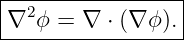
The two methods agree, verifying

------------------ | 2 | ∇--ϕ-=--∇-⋅ (∇-ϕ).

(53)

Solution 3: Laplace’s equation

For

ψ = x2 − y2, 1

(54)

we have

∇2 ψ1 = 2 − 2 + 0 = 0.

(55)

Thus

|------------------------------| |ψ1 satisfies Laplace’s equation.| --------------------------------

(56)

For

ψ = x2 + y2 + z2, 2

(57)

we obtain

2 ∇ ψ2 = 2 + 2 + 2 = 6.

(58)

Therefore,

|--------------------------------------| -ψ2-does-not-satisfy-Laplace’s-equation.-

(59)

For

ψ3 = xy + yz + zx,

(60)

all pure second derivatives vanish, so

|----------| -∇2ψ3-=--0.-

(61)

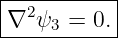
Hence ψ₃ also satisfies Laplace’s equation.

Solution 4: reduction from 3D to 1D

The Cartesian Laplacian is

∇2 ψ = ψ + ψ + ψ . xx yy zz

(62)

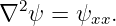
If ψ depends only on x and t, then

ψ = 0, ψ = 0, y z

(63)

and therefore

ψyy = 0, ψzz = 0.

(64)

Thus

∇2 ψ = ψxx.

(65)

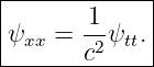
Substituting into the 3D wave equation gives

|------------| | -1 | |ψxx = c2ψtt.| --------------

(66)

This is exactly the one-dimensional wave equation developed in the Wave mechanics series.

Solution 5: verify a plane-wave solution

Let

𝜃 = k ⋅ r − ωt,

(67)

so that

ψ = A cos 𝜃.

(68)

Because

∇ 𝜃 = k,

(69)

the gradient is

∇ ψ = − A sin 𝜃k.

(70)

Taking one more spatial derivative gives

|--------------| |∇2 ψ = − k2ψ. | ---------------

(71)

For time derivatives,

ψ = A ω sin 𝜃 t

(72)

and

|------------| | 2 | -ψtt =-−-ω-ψ.-

(73)

Substitute these into

2 1 ∇ ψ = c2ψtt :

(74)

ω2 − k2ψ = − --2 ψ. c

(75)

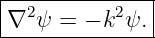
For a nonzero wave field,

2 k2 = ω-. c2

(76)

Taking the positive-frequency branch gives

|--------| -ω-=-ck.-|

(77)

Solution 6: wave vector, wavelength, and frequency

The wave vector is

k = (3xˆ+ 4ˆy)rad/m.

(78)

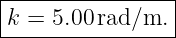
Its magnitude is

√ -2----2 k = 3 + 4 = 5.00rad/m.

(79)

Therefore,

|----------------| -k-=-5.00rad/m.--|

(80)

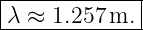
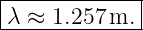
The wavelength is

2π 2π λ = --- = ---- ≈ 1.257 m. k 5.00

(81)

Thus

|------------| λ-≈--1.257m.--

(82)

The angular frequency is

ω = ck = (2.00 × 108)(5.00 ) = 1.00 × 109 rad/s.

(83)

Hence

|---------------------| ω = 1.00 × 109rad/s. | ----------------------

(84)

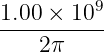
The ordinary frequency is

f	=	(85)
	=	(86)
	≈ 1.5915 × 10⁸ Hz.	(87)

Therefore,

|------------------------------| |f ≈ 1.59 × 108 Hz = 159 MHz. | -------------------------------

(88)

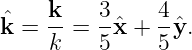
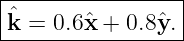
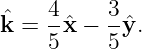
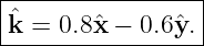
The unit propagation direction is

ˆ k- 3- 4- k = k = 5ˆx + 5 ˆy.

(89)

Thus

|----------------| -ˆk =-0.6ˆx-+-0.8ˆy.-

(90)

Solution 7: wavelength of a GPS-frequency radio wave

Use

λ = c. f

(91)

With

c = 299792458 m/s

(92)

and

f = 1.57542 × 109 Hz,

(93)

we obtain

--299792458--- λ = 1.57542 × 109 ≈ 0.190294 m.

(94)

Thus

|-------------------------| λ-≈--0.1903-m--=-19.03-cm.--

(95)

The scalar wavenumber is

2π 2π k = ---≈ ---------≈ 33.02 rad/m. λ 0.190294

(96)

Therefore,

|----------------| k-≈--33.02-rad/m.--

(97)

Solution 8: arbitrary traveling profile in three dimensions

Let

s = ˆn ⋅ r − ct

(98)

and

ψ = F (s).

(99)

Because n is constant,

∇s = ˆn.

(100)

Then

′ ∇ ψ = F (s)nˆ.

(101)

Taking the divergence,

∇2ψ = ∇ ⋅ (F ′(s )nˆ).

(102)

Since n is constant,

∇2 ψ = F ′′(s)|ˆn|2.

(103)

Because n is a unit vector,

|--------------| |∇2 ψ = F ′′(s).| ---------------

(104)

For time derivatives,

ψt = − cF ′(s)

(105)

and

|--------------| |ψ = c2F ′′(s).| --tt------------

(106)

Therefore,

1- ′′ 2 c2ψtt = F (s ) = ∇ ψ.

(107)

Hence any sufficiently smooth profile of the form

|----------------------| -ψ(r,t)-=-F-(ˆn-⋅ r −-ct)|

(108)

satisfies the three-dimensional wave equation.

Solution 9: the radial Laplacian

Let

1- ψ(r) = r .

(109)

Then

d-ψ -1 dr = − r2.

(110)

Multiply by r²:

dψ r2--- = − 1. dr

(111)

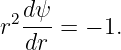
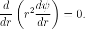
Differentiate again:

( ) d-- r2d-ψ = 0. dr dr

(112)

Therefore, for r > 0,

|--(---)------| ∇2 1- = 0. | | r | ---------------

(113)

The restriction r > 0 matters because 1∕r is singular at the origin.

Solution 10: spherical-wave amplitude spreading

For an outgoing spherical wave,

1 A(r) ∝ -. r

(114)

Thus

A r --2 = -1 . A1 r2

(115)

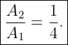
Since r₂ = 4r₁,

|--------| |A2- 1-| |A = 4.| --1-------

(116)

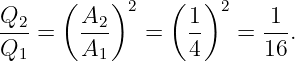
If another quantity is proportional to amplitude squared, then

( )2 ( )2 Q2-= A2- = 1- = 1-. Q1 A1 4 16

(117)

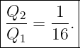
Hence

|----------| |Q2 1 | |--- = ---.| -Q1----16--

(118)

This is the mathematical precursor of inverse-square power-density spreading discussed later in the RF sequence.

Solution 11: reduce a spherical wave to a 1D radial equation

Begin with

1 ∂ ( ) 1 --2--- r2ψr = 2-ψtt. r ∂r c

(119)

Define

χ = rψ,

(120)

so that

χ- ψ = r .

(121)

Differentiate with respect to r:

χr χ ψr = ---− -2. r r

(122)

Multiply by r²:

2 r ψr = rχr − χ.

(123)

Differentiate again:

∂ ---(r2ψr ) = χr + rχrr − χr = rχrr. ∂r

(124)

Thus the left side becomes

1-(rχ ) = 1χ . r2 rr r rr

(125)

Because r is independent of time,

1- ψtt = r χtt.

(126)

Therefore,

1-χ = 1-1-χ . r rr c2r tt

(127)

For r > 0, multiply by r:

|------------| | 1 | |χrr = -2χtt.| -------c-----

(128)

So the transformed quantity χ = rψ obeys the ordinary 1D wave equation in the radial coordinate.

Solution 12: vector wave equation component by component

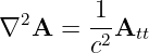
The vector equation

∇2A = 1-A c2 tt

(129)

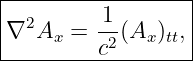
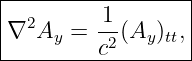
means that each Cartesian component obeys its own scalar wave equation:

|------------------| | 1 | |∇2Ax = -2(Ax)tt,| ----------c--------

(130)

|------------------| | 2 1- | |∇ Ay = c2(Ay)tt,| -------------------

(131)

and

|------------------| |∇2Az = 1-(Az)tt. | ----------c2-------|

(132)

For

A = A0 ˆy cos(kz − ωt),

(133)

only the y component is nonzero:

Ay = A0 cos(kz − ωt).

(134)

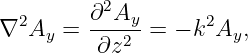
Its spatial Laplacian is

∂2A ∇2Ay = ----y = − k2Ay, ∂z2

(135)

while

2 (Ay )tt = − ω Ay.

(136)

Thus the component equation requires

2 k2 = ω-, c2

(137)

|--------| -ω-=-ck.-|

(138)

The x and z component equations are satisfied trivially because those components are zero.

Solution 13: identify which functions satisfy the 1D wave equation

For

u = A cos(kx − ckt), 1

(139)

we have angular frequency ω = ck, so the required relation is satisfied. Therefore,

|------------------------------| -u1-satisfies-the-wave-equation.-|

(140)

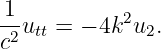
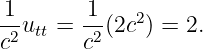
For

u2 = A cos(kx − 2ckt),

(141)

we have ω = 2ck. Then

2 uxx = − k u2

(142)

but

1 -2utt = − 4k2u2. c

(143)

These are not equal, so

|--------------------------------------| |u2 does not satisfy the wave equation. | ---------------------------------------

(144)

For

u = F (x − ct), 3

(145)

the chain rule gives

uxx = F′′(x − ct)

(146)

and

utt = c2F ′′(x − ct).

(147)

Therefore,

|------------------------------| |u satisfies the wave equation. | --3----------------------------

(148)

For

2 22 u4 = x + ct ,

(149)

we find

uxx = 2

(150)

and

1 1 2 -2utt = -2(2c ) = 2. c c

(151)

Thus

|----------------------------------| -u4-also-satisfies-the-wave--equation.-

(152)

This last result is a useful reminder: not every solution of the wave equation must look sinusoidal or like a localized traveling pulse.

Solution 14: synthesis - geometry, phase, wavelength, and frequency

The wave vector is

k = (4xˆ− 3ˆy)rad/m.

(153)

Its magnitude is

∘ ----------- k = 42 + (− 3)2 = 5.00rad/m.

(154)

Thus

|----------------| -k-=-5.00rad/m.--|

(155)

The unit propagation direction is

4 3 ˆk = --ˆx − -yˆ. 5 5

(156)

Therefore,

|----------------| kˆ= 0.8ˆx − 0.6ˆy.| ------------------

(157)

The wavelength is

2π 2π λ = -k-= -5-≈ 1.257 m.

(158)

Thus

|------------| λ-≈--1.257m.--

(159)

The angular frequency follows from ω = ck:

ω = (3.00 × 108)(5.00) = 1.50 × 109rad/s.

(160)

Hence

|---------------------| ω = 1.50 × 109rad/s. | ----------------------

(161)

The ordinary frequency is

f = ω--≈ 2.387 × 108 Hz. 2π

(162)

Therefore,

|------------------------------| |f ≈ 2.39 × 108 Hz = 239 MHz. | -------------------------------

(163)

r = (1,2,0)m,

(164)

we have

k ⋅ r = 4(1) − 3 (2 ) = − 2 rad.

(165)

−9 t = 2.0 ns = 2.0 × 10 s,

(166)

9 − 9 ωt = (1.50 × 10 )(2.0 × 10 ) = 3.00 rad.

(167)

Therefore the phase is

𝜃	= k ⋅ r − ωt + ϕ₀	(168)
	= −2 − 3 +	(169)
	≈−4.215 rad.	(170)

Thus

|----------------| -𝜃-≈-−-4.215rad.-|

(171)

Adding any integer multiple of 2π gives an equivalent phase representation.

Common mistakes

Confusing the vector k with its magnitude k = |k|.
Forgetting one or more Cartesian second derivatives when computing ∇²ψ.
Treating ∇² as an ordinary algebraic square rather than a differential operator.
Using ω = ck without checking that the governing wave equation is nondispersive with speed c.
Forgetting that 1∕r is singular at r = 0 when evaluating its Laplacian.
Forgetting the 1∕r amplitude factor in the usual outgoing spherical-wave solution.
Assuming every solution of the wave equation must be sinusoidal.

What EM04E reinforces

The central operator is

|-----------------------| ∇2 ψ = ψ + ψ + ψ | ---------xx----yy----zz-

(172)

with

|-----------------| | 2 | ∇--ψ-=--∇-⋅ (∇-ψ).-

(173)

The scalar 3D wave equation is

--------------- | 1 | |∇2 ψ = -2ψtt.| ---------c-----|

(174)

For a plane wave,

|-------| ω-=--ck-|

(175)

leads directly to

|--------| -c-=-fλ.-|

(176)

For spherical waves,

|--------------------| | 1- | |ψ(r,t) = rF (r − ct)| ----------------------

(177)

introduces the geometric spreading that later becomes central to radio link budgets and the Friis equation.

The next main lesson, EM05, introduces Electric Charge and the electric field.

References

[1] H. M. Schey, Div, Grad, Curl, and All That, 4th ed., W. W. Norton & Company, 2005.

[2] David J. Griffiths, Introduction to Electrodynamics, 4th ed., Cambridge University Press, 2017.

[3] Walter A. Strauss, Partial Differential Equations: An Introduction, 2nd ed., Wiley, 2007.

[4] Gilbert Strang and Edwin “Jed” Herman, Calculus, Volume 3, OpenStax, 2016, chapters on vector calculus and second-order differential operators.

[5] Samuel J. Ling, Jeff Sanny, and William Moebs, University Physics, Volume 2, OpenStax, 2016, chapters on electromagnetic waves.

[6] Frank S. Crawford, Jr., Waves, Berkeley Physics Course, Volume 3, McGraw-Hill, 1968.

[7] Massachusetts Institute of Technology, 8.03SC Physics III: Vibrations and Waves, MIT OpenCourseWare, materials on wave equations and traveling waves.

"Antennas Electromagnetic Waves" is owned by bloftin.
(view preamble)