Electromagnetic Waves, Antennas, and RF Examples: From a 1D Wave to a Field
This companion article provides self-study exercises for EM01, From a 1D wave to a field. The
exercises remain deliberately within the conceptual scope of EM01: scalar and vector fields, spatial
and temporal dependence, field components, field magnitude, snapshots, time histories, simple
vector waves, and local measurements. Gradient, divergence, curl, dot products, cross products,
and Maxwell’s equations are reserved for later lessons.
All exercises are stated first. Complete worked solutions follow in Part II.
The central conceptual bridge is
A scalar field assigns one scalar value to each point in its domain. A vector field assigns a vector to
each point. A fixed-location sensor samples a field through time as
These ideas are the mathematical starting point for later radio-wave, antenna, and GPS analysis
[1, 2, 3, 4].
How to use this problem set
Attempt all exercises in Part I before reading Part II. For every field expression, ask four questions
in order:
- What are the independent variables?
- Does the field return a scalar or a vector?
- Which directions describe the vector itself?
- Which coordinates describe where the field changes?
Keeping these questions separate avoids many early errors when reading electromagnetic wave
notation.
Part I: Exercises
Exercise 1: Scalar field or vector field?
The figure below contrasts the two basic possibilities introduced in EM01.
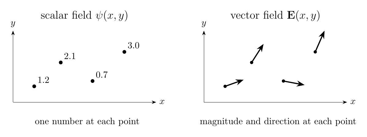
Figure. A scalar field assigns one number to each point. A vector field assigns a vector
with magnitude and direction to each point.
Classify each expression as scalar-valued or vector-valued:
| ψ(x,y) | = 3x − y, | (3)
|
| T(x,y,z,t) | = T0 + az, | (4)
|
| E(x,y) | = (2x)x + (y)y, | (5)
|
| p(x,t) | = p0 cos(kx − ωt), | (6)
|
| A(z,t) | = yA0 sin(kz − ωt). | (7) |
For each vector field, identify the basis directions that appear explicitly.
Exercise 2: Evaluate a scalar field
Let
Find the field value at
Is the result a scalar or a vector?
Exercise 3: Evaluate a vector field and its magnitude
Let
At
find:
- Ex, Ey, and Ez;
- the vector E;
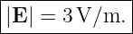
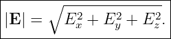
- the magnitude |E|.
Exercise 4: A one-dimensional wave is already a field
Consider
Explain why this is a scalar field even though it depends on two independent variables.
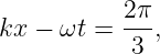
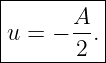
Then evaluate u∕A when
Exercise 5: Snapshot versus time history
The two panels below show two different views of the same wave field.
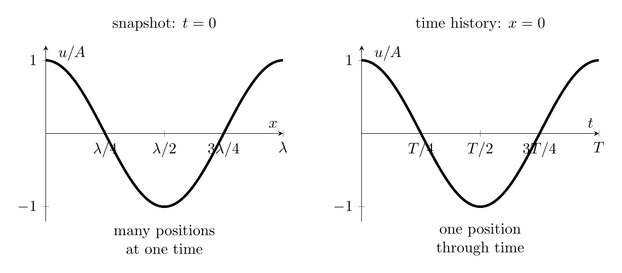
Figure. A spatial snapshot holds time fixed; a time history holds position fixed.
For
find:
- the spatial snapshot at t = 0;
- the time history at x = 0;
- the time history at a general fixed location x = x0.
Explain in words what is held fixed in each case.
Exercise 6: Position vector and compact field notation
A point in space has coordinates
- Write its position vector r.
- Compute |r|.
- Explain what the notation E(r,t) means in terms of x, y, and z.
Exercise 7: Uniform or nonuniform?
Classify each field as spatially uniform or spatially nonuniform at a fixed time:
| E1(r,t) | = E0 cos(ωt)x, | (16)
|
| E2(z,t) | = E0 cos(kz − ωt)x, | (17)
|
| ψ3(x,y) | = 5, | (18)
|
| ψ4(x,y) | = x2 + y2. | (19) |
Which expressions can still vary with time even when they are spatially uniform?
Exercise 8: Field direction versus propagation direction
Consider
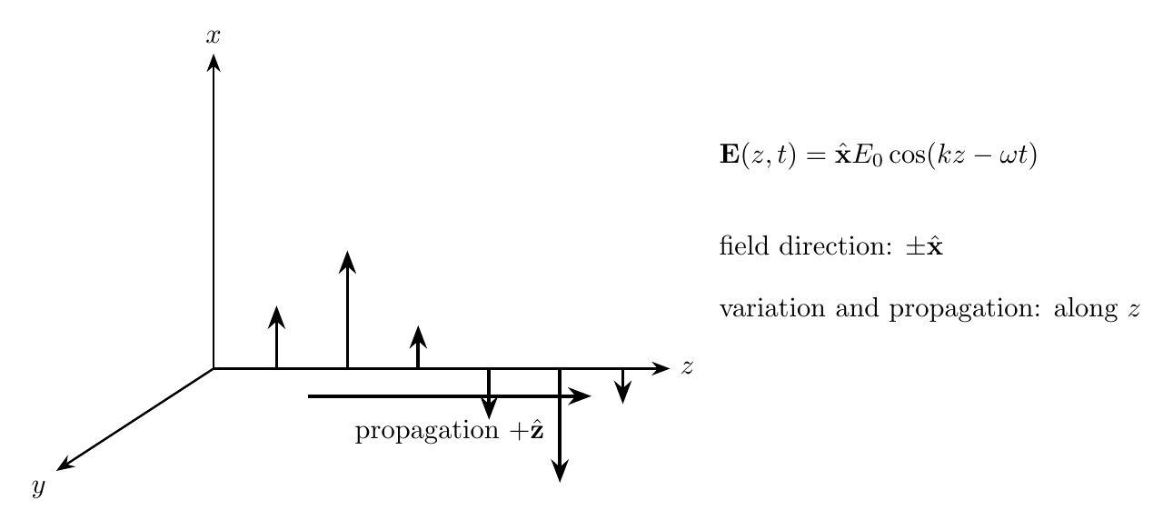
Figure. The field vector points along the x direction while the phase varies and propagates
along z.
Identify:
- the axis along which the field vector points;
- the direction in which the wave pattern propagates;
- the coordinate along which the phase varies;
- whether the field and propagation directions are parallel or perpendicular.
Exercise 9: Evaluate a vector wave at selected phases
Let
Find E and |E| when the phase is
- 0;
- π∕2;
- π;
- 3π∕2.
Explain the physical meaning of a negative x component.
Exercise 10: Read vector components from notation
Consider
At
find:
- all three components;
- the complete vector;
- the vector magnitude.
Exercise 11: A sensor samples a field locally
The figure below represents a spatially varying vector field and a sensor fixed at one
location.
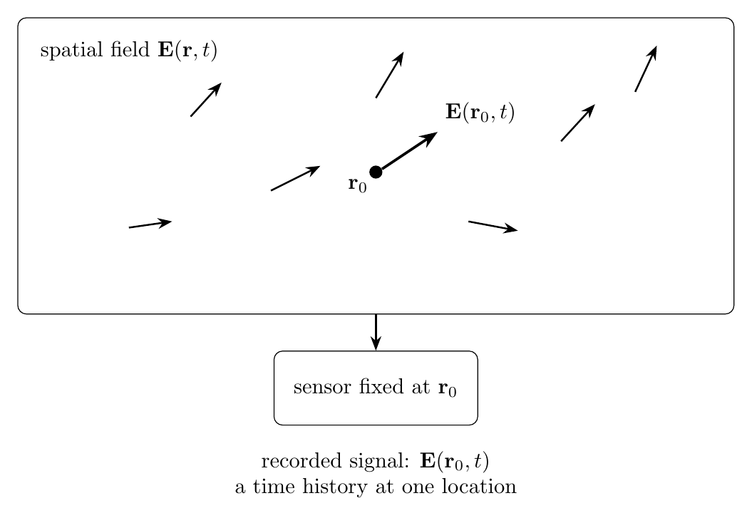
Figure. A sensor fixed at r0 records the local field through time as E(r0,t).
Suppose
A sensor is fixed at x = x0.
- Write the time history measured at the sensor.
- What variable still changes in that measured expression?
- Does this one sensor, by itself, provide the entire spatial field at one instant? Explain.
Exercise 12: Contours are not trajectories
A scalar field is
- Find the field value at (3, 4).
- Write the equation of the contour on which ψ = 25.
- Describe the geometric shape of that contour.
- Explain why the contour does not represent a material object or a field vector moving
along that curve.
Exercise 13: Same field, different questions
Let
Find:
- the spatial snapshot at t = 0;
- the time history at (x,y) = (2, 3);
- the field value at (x,y,t) = (2, 3,π∕(2ω));
- whether ψ is scalar-valued or vector-valued.
Exercise 14: Synthesis - read a three-dimensional vector field
Consider the illustrative field
At an event where
find:
- Ex, Ey, and Ez;
- the complete vector E;
- the magnitude |E|;
- which spatial coordinate appears in the phase;
- whether the field vector points along the same direction as the coordinate of variation
at this event.
Repeat parts (a)–(c) when
Explain what this example teaches about separating vector direction from spatial dependence.
Part II: Complete Worked Solutions
Solution 1: Scalar field or vector field?
The classification depends on what each function returns, not on how many independent variables
it has.
-
returns one number, so it is a scalar field.
-
returns one temperature value, so it is a scalar field.
-
contains basis directions and returns a vector. It is a vector field with explicit x and y
components.
-
returns one pressure value, so it is a scalar field.
-
is vector-valued. Its explicit basis direction is y.
Thus the number of coordinates in the argument does not decide whether a field is scalar or
vector-valued.
Solution 2: Evaluate a scalar field
Substitute
into
Then
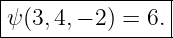
| ψ(3, 4,−2) | = 2(3) − 4 + (−2)2 | (37)
|
| = 6 − 4 + 4 | (38)
|
| = 6. | (39) |
Therefore
The result is a scalar because the field itself is scalar-valued.
Solution 3: Evaluate a vector field and its magnitude
The components are
At (1,−2, 2),
| Ex | = 2, | (42)
|
| Ey | = −(−2) = 2, | (43)
|
| Ez | = 3(2) = 6. | (44) |
Hence
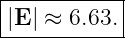
The magnitude is
| |E| | =  | (46)
|
| =  | (47)
|
| ≈ 6.63. | (48) |
Therefore
Solution 4: A one-dimensional wave is already a field
The function
assigns one scalar value u to every pair (x,t). It is therefore a scalar field on one spatial dimension
plus time.
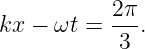
At phase
we have
Thus
The fact that u depends on two variables does not make it vector-valued.
Solution 5: Snapshot versus time history
Starting from
set t = 0 for a spatial snapshot:
This compares many positions at one instant.
Set x = 0 for a time history at the origin:
| u(0,t) | = A cos(−ωt) | (57)
|
| = A cos(ωt), | (58) |
because cosine is even. Thus
At a general fixed location x = x0,
The snapshot holds time fixed. The time history holds position fixed.
Solution 6: Position vector and compact field notation
The position vector is
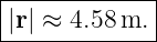
Its magnitude is
| |r| | =  m m | (62)
|
| =  m m | (63)
|
| ≈ 4.58 m. | (64) |
Therefore
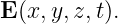
The notation
is compact notation for a vector field whose spatial dependence can be written as
The symbol r packages the three spatial coordinates into one position vector.
Solution 7: Uniform or nonuniform?
For
there is no spatial coordinate in the value, so the field is spatially uniform. It can still vary with
time.
For
the value changes with z, so it is spatially nonuniform.
For
the value is the same everywhere, so the field is spatially uniform.
For
the value changes from point to point, so the field is spatially nonuniform.
Thus
while
Only E1 among the spatially uniform examples explicitly varies with time.
Solution 8: Field direction versus propagation direction
The field is
The basis vector x tells us that the field vector lies along the x axis. Depending on the sign of the
cosine, it points toward +x or −x.
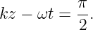
The phase
has the right-moving form, so the pattern propagates toward increasing z.
The spatial coordinate appearing in the phase is z, so the phase varies along the z direction.
Therefore
These directions are perpendicular in this illustrative transverse wave.
Solution 9: Evaluate a vector wave at selected phases
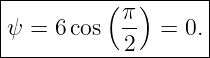
The field is
where
At 𝜃 = 0,
so
At 𝜃 = π∕2,
At 𝜃 = π,
At 𝜃 = 3π∕2,
A negative x component means the vector points in the −x direction. It does not mean the vector
magnitude is negative.
Solution 10: Read vector components from notation
The components are
At
we get
| Fx | = 2 + 0.5 = 2.5, | (87)
|
| Fy | = 2(−1) = −2, | (88)
|
| Fz | = −3(0.5) = −1.5. | (89) |
Thus
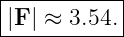
The magnitude is
| |F| | =  | (91)
|
| =  | (92)
|
| ≈ 3.54. | (93) |
Therefore
Solution 11: A sensor samples a field locally
The full field is
At the fixed sensor position x = x0,
The position x0 is now a constant. Time t remains the changing independent variable.
A single sensor therefore records a time history at one location. It does not, by itself, give the
complete spatial field at one instant because values at other positions are not simultaneously
measured.
Solution 12: Contours are not trajectories
The field is
At (3, 4),
| ψ(3, 4) | = 32 + 42 | (98)
|
| = 9 + 16 | (99)
|
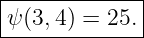
| = 25. | (100) |
Thus
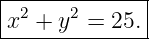
The contour ψ = 25 satisfies
This is a circle of radius 5 centered at the origin.
The contour simply identifies all points where the scalar field has the same value. It is not, by
itself, the path of a particle, a material object, or a vector arrow moving through the
field.
Solution 13: Same field, different questions
The scalar field is
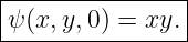
At t = 0,
so the spatial snapshot is
At the fixed point (2, 3),
At
we have
so
The field is scalar-valued because it returns one number for each (x,y,t).
Solution 14: Synthesis - read a three-dimensional vector field
The field is
with
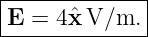
At 𝜃 = 0,
Therefore
and
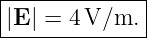
Its magnitude is
The only spatial coordinate appearing in the phase is z, so the field varies spatially
along z in this expression. At this event, the vector itself points along x, not along
z.
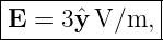
At
we have
Thus
so
with
The field direction can change even though the spatial dependence still enters through the
coordinate z. This is exactly why vector direction and direction of spatial variation must be read
separately from the notation.
Common mistakes
- Mistake: deciding that a field is vector-valued merely because it depends on several
variables. Scalar fields can depend on many spatial coordinates and time.
- Mistake: confusing a negative vector component with a negative magnitude.
Magnitude is nonnegative; the sign belongs to a component direction.
- Mistake: confusing the basis direction of a vector with the coordinate along which the
field varies.
- Mistake: treating a spatial snapshot and a time history as the same graph. One holds
time fixed; the other holds position fixed.
- Mistake: interpreting contour lines as trajectories. They only connect equal scalar-field
values.
- Mistake: assuming one fixed sensor measures the entire spatial field at one instant.
What EM01E reinforces
The exercises reinforce the sequence
A scalar field returns one scalar value at each event. A vector field returns a vector with
components such as
Its magnitude is
A field’s vector direction and its direction of spatial variation are separate ideas. A fixed sensor
samples the field locally as
These concepts prepare the way for EM02, where the vector mathematics will be developed more
systematically before Maxwell’s equations are introduced.
References
[1] David J. Griffiths, Introduction to Electrodynamics, 4th ed., Cambridge University
Press, 2017.
[2] Samuel J. Ling, Jeff Sanny, and William Moebs, University Physics, Volume 2,
OpenStax, 2016, chapters on electric fields, magnetic fields, and electromagnetic waves.
[3] Richard P. Feynman, Robert B. Leighton, and Matthew Sands, The Feynman Lectures
on Physics, Volume II, Addison-Wesley, 1964, chapters introducing electromagnetic
fields.
[4] Massachusetts Institute of Technology, 8.02 Physics II: Electricity and Magnetism,
MIT OpenCourseWare, materials on electric and magnetic fields.
[5] Frank S. Crawford, Jr., Waves, Berkeley Physics Course, Volume 3, McGraw-Hill,
1968.

![[parent]](https://images.physicslibrary.org/images/uparrow.png)