Calculus of Variations: Higher-Order Variational Problems
Up to CV07, the basic integral functional depended on a function and its first derivative,
Many important physical models depend on higher derivatives. Bending energy depends on
curvature and therefore, in a small-slope beam model, on y′′. Smooth trajectory design can
penalize acceleration or jerk. Higher-gradient field theories and regularization methods likewise
introduce derivatives beyond first order. The calculus of variations handles these problems by the
same central idea used before: vary the function, integrate derivatives off the variation, and apply
the Fundamental Lemma. The new feature is that integration by parts must be repeated. Standard
treatments are given in [1, 2, 3].
This article develops the classical higher-order Euler–Lagrange equation, with particular attention
to the second-order case
because it already contains the essential structure: a fourth-order differential equation and two
independent endpoint variations, η and η′.
1 Why higher derivatives change the problem
Suppose the functional contains y′′. A perturbation
implies
Therefore the first variation contains three kinds of terms:
The term multiplying η′ requires one integration by parts. The term multiplying η′′ requires two.
This repeated transfer of derivatives is the source of both the higher-order Euler–Lagrange
equation and the enlarged boundary-term structure.

Figure. The Fy′′η′′ term must be integrated by parts twice. The interior contribution is
reduced to a coefficient multiplying η, while the endpoint contribution retains both η and
η′.
2 Admissible variations for a second-order problem
There are several possible endpoint specifications. The cleanest theorem first fixes both the value
and slope at each endpoint:
An admissible variation must preserve all four conditions. Thus
and
This is the higher-order analogue of the fixed-endpoint condition in CV04. Because a fourth-order
differential equation will emerge, four scalar boundary conditions are also exactly what is normally
needed to determine a unique classical solution.
3 Derivation for F(x,y,y′,y′′)
Start from
Integrate the Fy′η′ term once:
Now integrate the Fy′′η′′ term once:
The remaining integral still contains η′, so integrate by parts again:
Collect the endpoint terms and the interior terms:
| δJ | = ![[ ( ) ]
F ′ −-d-F ′′ η + F ′′η′
y dx y y](https://images.physicslibrary.org/cache/objects/1205/make4ht/CalculusOfVariationsHigherOrderVariationalProblems12x.png) ab ab | (13)
|
| + ∫
ab![[ 2 ]
Fy − -d-Fy′ + -d--Fy′′
dx dx2](https://images.physicslibrary.org/cache/objects/1205/make4ht/CalculusOfVariationsHigherOrderVariationalProblems13x.png) η dx. η dx. | (14) |
This formula is worth separating into two pieces:
and
If y and y′ are fixed at both endpoints, then η = η′ = 0 there, so the complete boundary term
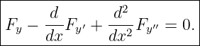
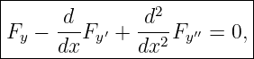
vanishes. Stationarity for every admissible η gives
By the Fundamental Lemma,
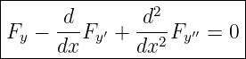
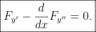
This is the second-order Euler–Lagrange equation.
4 Classical theorem for second-order functionals
Theorem. Let
with F sufficiently smooth, and suppose y∗ is a sufficiently smooth local extremum among
admissible functions satisfying fixed values of y and y′ at a and b. Then y∗ satisfies
throughout the interior of the interval.
Proof. The local-extremum hypothesis implies δJ[y∗; η] = 0 for every admissible variation.
The two integrations by parts derived above produce the boundary term and interior
term. Fixed y and y′ imply η = η′ = 0 at both endpoints, eliminating the boundary
term. The Fundamental Lemma then forces the interior coefficient to vanish pointwise.
□
As before, this theorem supplies a necessary stationarity condition. It does not by itself prove that
a solution is a minimum.
5 The general nth-order Euler–Lagrange equation
Now consider
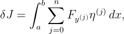
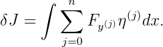
The first variation is
where y(0) = y and η(0) = η.
Integrating the term containing η(j) by parts exactly j times transfers all derivatives from η onto
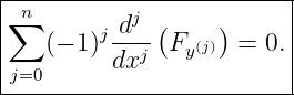
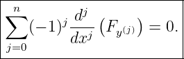
Fy(j). The interior result is
Written out,
The alternating signs are not arbitrary. Each integration by parts introduces one minus
sign.
For completely fixed endpoint data through derivative order n − 1, the admissible variations
satisfy
6 The general boundary structure
Repeated integration by parts also produces the boundary expression
This formula looks complicated, but its meaning is simple: an nth-order variational problem can
contain the independent endpoint variations
If any corresponding endpoint datum is free, the coefficient multiplying that independent variation
must satisfy a natural boundary condition.
7 Natural boundary conditions in the second-order case
Return to
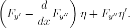
At a free endpoint the boundary expression is
If both y and y′ are free there, then η and η′ are independently arbitrary. Therefore stationarity
requires
and
If only y is free but y′ is fixed, then only the second condition involving the coefficient of η is
required. If only y′ is free, then only Fy′′ = 0 is required.
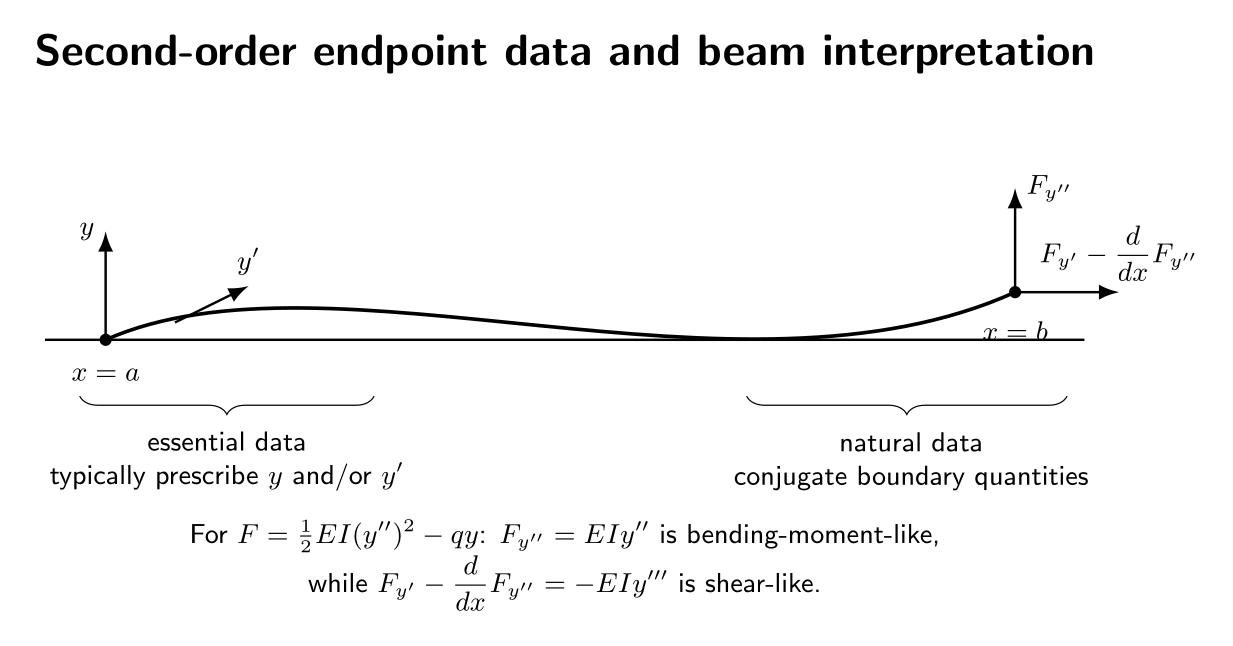
Figure. A second-order functional has two independent endpoint variation channels. In
beam language, fixing displacement and slope corresponds to essential data, while the two
conjugate coefficients become moment-like and shear-like natural data.
8 Example: pure curvature energy
Consider
subject to
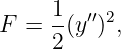
Here
so
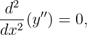
The second-order Euler–Lagrange equation gives
or
Therefore every stationary curve is cubic:
Apply the four endpoint conditions. From y(0) = 0 and y′(0) = 0,
The two conditions at x = 1 give
| C + D | = 1, | (40)
|
| 2C + 3D | = 0. | (41) |
Solving,
Hence
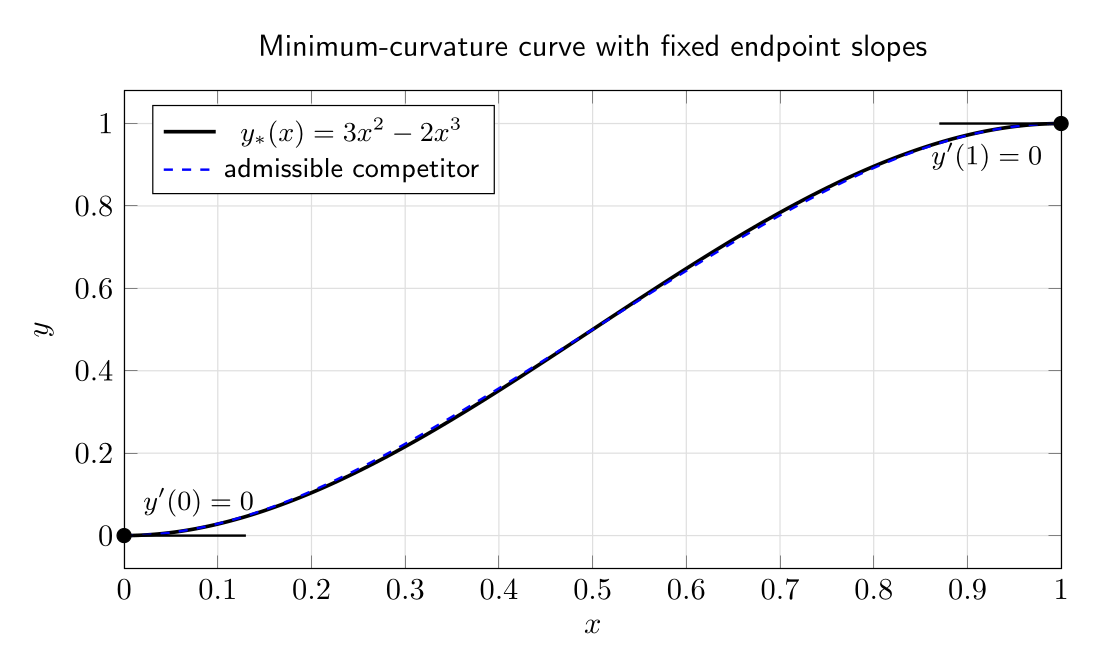
Figure. The stationary curve for the quadratic curvature functional is cubic. The endpoint
values and endpoint slopes provide the four conditions required by the fourth-order
Euler–Lagrange equation.
8.1 Why this stationary curve is actually the unique global minimum
Let any admissible competitor be written
where
Then
| J[y] | =  ∫
01(y
∗′′ + η′′)2dx ∫
01(y
∗′′ + η′′)2dx | (46)
|
| = J[y∗] + ∫
01y
∗′′η′′dx +  ∫
01(η′′)2dx. ∫
01(η′′)2dx. | (47) |
Integrating the cross term twice gives
The boundary term vanishes because η = η′ = 0, and the interior term vanishes because y∗′′′′ = 0.
Thus
Equality requires η′′ = 0, so η is linear. The four homogeneous endpoint conditions
then force η ≡ 0. Therefore the cubic is the unique global minimizer in this admissible
class.
9 Connection to Euler–Bernoulli beam bending
For a slender beam in the small-deflection approximation, a standard potential-energy functional is
[5]
where E is Young’s modulus, I is the second moment of area, and q(x) is a distributed transverse
load.
Here
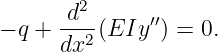
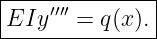
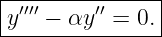
for constant EI. The higher-order Euler–Lagrange equation becomes
For constant flexural rigidity,
This fourth-order beam equation is therefore not an unrelated engineering formula; it is a direct
Euler–Lagrange equation for bending energy minus load potential.
At a free beam end, both η and η′ are unrestricted. The natural conditions are
and
Up to sign convention, these are zero bending moment and zero shear force. This gives a physical
interpretation to the abstract higher-order boundary coefficients.
10 Mixed essential and natural boundary conditions
Consider the beam functional above with the left end clamped:
and the right end free. At x = 0,
so no natural conditions are generated there. At x = L, η(L) and η′(L) are arbitrary,
so
and
The fourth-order differential equation therefore receives two essential conditions at the clamped
end and two natural conditions at the free end.
This counting principle is useful:
A classical 2nth-order Euler–Lagrange equation normally needs 2n scalar
boundary conditions. Essential conditions prescribe endpoint data directly;
natural conditions arise from the surviving boundary variation.
11 Example: slope and curvature penalty
Consider
Then
Therefore
or
The characteristic equation is
so
Thus
Adding a first-derivative penalty changes the cubic minimum-curvature family into a combination
of polynomial and hyperbolic terms.
12 Third-order dependence: minimum jerk
A trajectory-design problem may penalize jerk, the third derivative of position. Consider
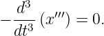
The integrand depends only on x′′′, so the n = 3 Euler–Lagrange equation is
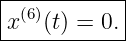
Hence
The stationary trajectory is therefore a polynomial of degree at most five.
Suppose position, velocity, and acceleration are fixed at both endpoints:
| x(0) | = 0, | ẋ(0) | = 0, | ẍ(0) | = 0, | (70)
|
| x(T) | = D, | ẋ(T) | = 0, | ẍ(T) | = 0. | (71) |
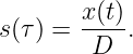
Introduce normalized time
and normalized position
Solving the six endpoint conditions gives
Thus
This quintic profile is widely known as the minimum-jerk trajectory. Minimum-jerk models also
have an important history in studies of smooth human movement [6].
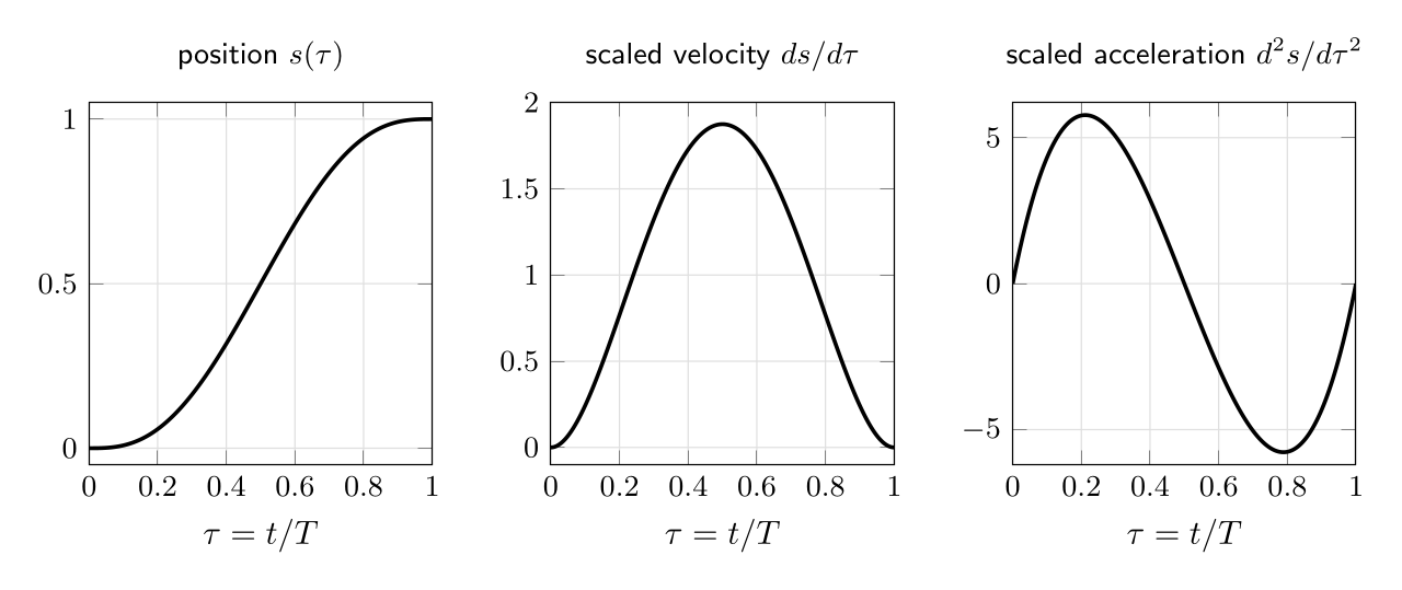
Figure. The normalized quintic minimum-jerk trajectory. Position, velocity, and
acceleration all satisfy the required endpoint values smoothly.
13 Higher-derivative mechanics
A mechanical action may depend on acceleration,
The stationarity condition is
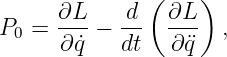
The boundary term is
This suggests two momentum-like quantities,
and
They are conjugate to endpoint variations in position and velocity, respectively. In advanced
hamiltonian formulations of nondegenerate higher-derivative mechanics these quantities lead
toward the Ostrogradsky construction, which has important stability implications. That subject
lies beyond the present classical variational derivation.
14 Regularity and order counting
The appearance of higher derivatives in the functional raises the regularity requirements. A
classical derivation assumes enough smoothness that all derivatives generated by repeated
integration by parts exist and are continuous as needed.
For
the Euler–Lagrange equation can contain y′′′′. Thus even though the original integrand explicitly
contains derivatives only through second order, the stationarity equation is generally fourth
order.
More generally, dependence on y(n) commonly produces a differential equation of order as high as
2n. Degeneracies can reduce the actual order. For example, if the integrand is linear rather than
quadratic in the highest derivative, cancellation may occur.
15 Necessary versus sufficient conditions
The generalized Euler–Lagrange equation remains a necessary condition for a smooth local
extremum under the stated assumptions. It is not automatically sufficient.
The pure curvature functional
was easy to classify because it is a positive quadratic functional, and the direct difference argument
established a global minimum. A general higher-order functional can be indefinite, nonconvex, or
degenerate. Classification requires second-variation and sufficiency theory, developed later in
CV11–CV13.
16 Common mistakes
- Stopping after one integration by parts. A term multiplying η′′ must be integrated
by parts twice before the Fundamental Lemma can be applied directly.
- Forgetting the η′ boundary term. A second-order functional has two independent
endpoint variation channels.
- Fixing y but silently assuming y′ is fixed. These are different admissible classes
and lead to different natural boundary conditions.
- Missing the alternating signs. The generalized equation contains (−1)j because
each integration by parts contributes another minus sign.
- Assuming second-order dependence gives a second-order ODE. Quadratic
dependence on y′′ typically produces a fourth-order Euler–Lagrange equation.
- Calling every fourth-order equation a beam equation. The beam interpretation
depends on the specific energy functional and constitutive model.
- Confusing stationarity with minimality. Higher-order Euler–Lagrange equations
still provide necessary conditions unless additional arguments are supplied.
17 A compact workflow
For a higher-order functional, use the following sequence:
- Identify the highest derivative y(n) appearing in F.
- Determine which endpoint values among y,y′,…,y(n−1) are fixed and which are free.
- Form the first variation
- Integrate the jth term by parts j times.
- Collect the interior coefficient of η.
- Apply the Fundamental Lemma to obtain the generalized Euler–Lagrange equation.
- Keep the complete boundary expression and use endpoint freedom to derive natural
conditions.
- Solve the resulting higher-order boundary-value problem.
- Separately determine whether the stationary solution is actually a minimum, maximum, or
saddle.
18 What CV09 adds
CV08 has enlarged the derivative order while keeping the admissible functions otherwise
unconstrained except for endpoint data. CV09 introduces a different complication: integral
constraints and isoperimetric conditions. Those problems require variational Lagrange multipliers
and an augmented integrand.
The conceptual progression is therefore
Summary
For
a smooth stationary function satisfies
For the important second-order case,
with boundary term
These formulas explain why bending-energy problems produce fourth-order equations, why free
beam ends produce moment and shear natural conditions, why minimum-curvature interpolation is
cubic, and why minimum-jerk trajectories are quintic.
References
[1] I. M. Gelfand and S. V. Fomin, Calculus of Variations, Dover Publications, 2000.
[2] Bruce van Brunt, The Calculus of Variations, Springer, 2004.
[3] Hans Sagan, Introduction to the Calculus of Variations, Dover Publications, 1992.
[4] Cornelius Lanczos, The Variational Principles of Mechanics, 4th ed., Dover
Publications, 1986.
[5] L. D. Landau and E. M. Lifshitz, Theory of Elasticity, 3rd ed.,
Butterworth-Heinemann, 1986.
[6] Tamar Flash and Neville Hogan, “The coordination of arm movements: an
experimentally confirmed mathematical model,” Journal of Neuroscience, Vol. 5, No. 7,
pp. 1688–1703, 1985.

![∫ b
J[y] = F (x,y,y′)dx.
a](https://images.physicslibrary.org/cache/objects/1205/make4ht/CalculusOfVariationsHigherOrderVariationalProblems0x.png)
![∫ b
J [y ] = F(x, y,y′,y ′′)dx,
a](https://images.physicslibrary.org/cache/objects/1205/make4ht/CalculusOfVariationsHigherOrderVariationalProblems1x.png)


![∫ b
δJ[y;η] = (F η + F ′η ′ + F ′′η′′) dx.
a y y y](https://images.physicslibrary.org/cache/objects/1205/make4ht/CalculusOfVariationsHigherOrderVariationalProblems4x.png)




![∫ b ∫ b
Fy ′η ′dx = [Fy′η ]b − d-Fy ′ ηdx.
a a a dx](https://images.physicslibrary.org/cache/objects/1205/make4ht/CalculusOfVariationsHigherOrderVariationalProblems9x.png)
![∫ b ∫ b
F ′′η ′′dx = [F ′′η ′]b− -d-F ′′ η ′dx.
a y y a a dx y](https://images.physicslibrary.org/cache/objects/1205/make4ht/CalculusOfVariationsHigherOrderVariationalProblems10x.png)
![∫ b d [ d ]b ∫ b d2
− --Fy ′′ η′dx = − ---Fy′′ η + ---2Fy′′ ηdx.
a dx dx a a dx](https://images.physicslibrary.org/cache/objects/1205/make4ht/CalculusOfVariationsHigherOrderVariationalProblems11x.png)
![|-----------------[-(------------)----------]b-|
| -d- ′ |
|boundary term = Fy ′ − dx Fy′′ η + Fy ′′η |
----------------------------------------------a-](https://images.physicslibrary.org/cache/objects/1205/make4ht/CalculusOfVariationsHigherOrderVariationalProblems14x.png)

![∫ [ ]
b d-- -d2-
Fy − dxFy ′ + dx2 Fy′′ ηdx = 0.
a](https://images.physicslibrary.org/cache/objects/1205/make4ht/CalculusOfVariationsHigherOrderVariationalProblems16x.png)
![∫ b
′ ′′
J[y] = a F (x,y,y ,y )dx](https://images.physicslibrary.org/cache/objects/1205/make4ht/CalculusOfVariationsHigherOrderVariationalProblems18x.png)
![∫ b ( )
J [y ] = F x,y,y′,...,y(n) dx.
a](https://images.physicslibrary.org/cache/objects/1205/make4ht/CalculusOfVariationsHigherOrderVariationalProblems20x.png)


![|------------------------------------|
|[ n j−1 ]b |
| ∑ ∑ k-dk-( ) (j−1− k) |
| (− 1) dxk Fy(j) η .|
--j=1-k=0-------------------------a--](https://images.physicslibrary.org/cache/objects/1205/make4ht/CalculusOfVariationsHigherOrderVariationalProblems25x.png)

![∫
b ′ ′′
J [y ] = F(x, y,y,y )dx.
a](https://images.physicslibrary.org/cache/objects/1205/make4ht/CalculusOfVariationsHigherOrderVariationalProblems27x.png)

![∫
1- 1 ′′ 2
J[y] = 2 (y ) dx
0](https://images.physicslibrary.org/cache/objects/1205/make4ht/CalculusOfVariationsHigherOrderVariationalProblems31x.png)









![∫ ∫
1 ′′′′ ′′ ′ ′′′ 1 1 ′′′′
y∗η dx = [y∗η − y ∗ η]0 + y∗ η dx.
0 0](https://images.physicslibrary.org/cache/objects/1205/make4ht/CalculusOfVariationsHigherOrderVariationalProblems45x.png)
![|----------------∫---------------|
| 1 1 ′′2 |
|J[y] − J[y∗] = 2 (η ) dx ≥ 0.|
------------------0--------------](https://images.physicslibrary.org/cache/objects/1205/make4ht/CalculusOfVariationsHigherOrderVariationalProblems46x.png)
![∫ L[ ]
Π[y] = 1EI (y′′)2 − q(x)y dx,
0 2](https://images.physicslibrary.org/cache/objects/1205/make4ht/CalculusOfVariationsHigherOrderVariationalProblems47x.png)







![∫ b
1- [ ′′ 2 ′2]
J[y] = 2 a (y ) + α (y) dx, α > 0.](https://images.physicslibrary.org/cache/objects/1205/make4ht/CalculusOfVariationsHigherOrderVariationalProblems57x.png)





![∫ T
J[x] = 1- (x ′′′(t))2dt.
2 0](https://images.physicslibrary.org/cache/objects/1205/make4ht/CalculusOfVariationsHigherOrderVariationalProblems64x.png)


![|---------[-------------------------------]--|
| ( t)3 ( t)4 ( t )5 |
|x(t) = D 10 -- − 15 -- + 6 -- .|
| T T T |
----------------------------------------------](https://images.physicslibrary.org/cache/objects/1205/make4ht/CalculusOfVariationsHigherOrderVariationalProblems70x.png)
![∫
tf
S [q] = L(t,q, ˙q, ¨q)dt.
t0](https://images.physicslibrary.org/cache/objects/1205/make4ht/CalculusOfVariationsHigherOrderVariationalProblems71x.png)

![[( ∂L d ∂L ) ∂L ]tf
--- − -- --- η + ---η˙ .
∂ ˙q dt ∂¨q ∂ ¨q t0](https://images.physicslibrary.org/cache/objects/1205/make4ht/CalculusOfVariationsHigherOrderVariationalProblems73x.png)


![∫
1- ′′2
J [y] = 2 (y )dx](https://images.physicslibrary.org/cache/objects/1205/make4ht/CalculusOfVariationsHigherOrderVariationalProblems77x.png)

![∫
b ( ′ (n))
J [y ] = F x,y,y ,...,y dx,
a](https://images.physicslibrary.org/cache/objects/1205/make4ht/CalculusOfVariationsHigherOrderVariationalProblems80x.png)
![|------------------------------|
|[( d ) ]b |
| Fy′ − ---Fy′′ η + Fy′′η′ .|
----------dx----------------a--|](https://images.physicslibrary.org/cache/objects/1205/make4ht/CalculusOfVariationsHigherOrderVariationalProblems83x.png)