Wave Mechanics: Right- and Left-Traveling Solutions

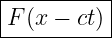
WM15 verified that every sufficiently smooth profile of the form

F (x − ct)

(1)

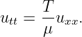
satisfies the one-dimensional wave equation

|-------2---| -utt =-cuxx-,

(2)

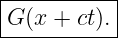
and that the same is true for every sufficiently smooth profile of the form

G(x + ct).

(3)

WM16 now asks the deeper structural question:

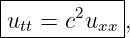
|--------------------------------------------------------------------------| -Why--does-the-wave--equation-naturally-contain-two-propagation--directions?-|

(4)

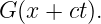
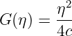
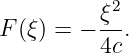
The answer is that the second-order wave operator can be separated into two first-order propagation operators. Those two operators correspond to information moving at speeds +c and −c. In characteristic coordinates, the wave equation then reduces to a particularly simple mixed-derivative equation whose sufficiently smooth solutions have the form

|--------------------------------| |u(x,t) = F (x − ct) + G (x + ct). ---------------------------------

(5)

This is the structural form underlying the classical d’Alembert solution of the one-dimensional wave equation [1, 2, 4, 6].

WM16 derives this two-family structure. WM17 will take the next step: given an initial displacement and initial velocity, determine the specific functions F and G.

1 One equation supports two directions

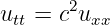
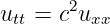
The homogeneous one-dimensional wave equation is

u − c2u = 0. tt xx

(6)

WM15 showed directly that

uR(x,t) = F (x − ct)

(7)

moves toward increasing x, while

uL(x,t) = G (x + ct)

(8)

moves toward decreasing x.

The two families are illustrated below.

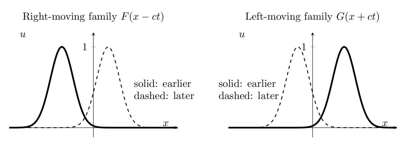
Figure. The same shape-preserving idea produces two propagation families. A profile depending on x − ct moves toward increasing x; a profile depending on x + ct moves toward decreasing x.

The speed magnitude is the same in both cases. Only the direction changes.

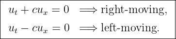
2 The first-order equations retain direction information

For a right-moving wave

uR (x,t) = F (x − ct),

(9)

WM15 found

ut = − cux.

(10)

Therefore

|----------------------------------------------| |u + cu = 0 for a pure right-moving wave. | --t-----x--------------------------------------

(11)

For a left-moving wave

uL (x,t) = G (x + ct),

(12)

we have

ut = +cux,

(13)

|--------------------------------------------| -ut −-cux-=-0----for-a pure-left- moving--wave.--

(14)

These are first-order transport equations. Unlike the second-order wave equation, they remember the propagation direction.

The distinction can be summarized as

|----------------------------------| | u + cu = 0 =⇒ right-moving, | | t x | | ut − cux = 0 =⇒ left- moving. | -----------------------------------

(15)

This interpretation is standard in treatments of traveling-wave solutions and characteristics [4, 6].

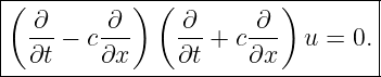
3 Factor the wave operator

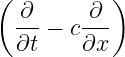
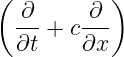
Because c is constant and the partial derivatives commute for a sufficiently smooth function, we may write

u	= u_tt + cu_tx − cu_xt − c²u_xx	(16)
	= u_tt − c²u_xx.	(17)

Thus the wave equation can be factored as

|(----------)-(----------)-------| | -∂- ∂-- ∂-- ∂-- | | ∂t − c∂x ∂t + c∂x u = 0.| ----------------------------------

(18)

This factorization is the PDE analogue of factoring an algebraic expression such as

2 2 a − b = (a − b)(a + b).

(19)

It hints that two first-order propagation mechanisms are embedded inside the second-order wave equation.

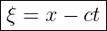
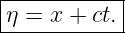
4 Characteristic coordinates

Introduce the coordinates

|----------| -ξ =-x-−-ct-

(20)

and

|----------| η-=-x-+--ct.-

(21)

The coordinate ξ stays constant along a right-moving feature. The coordinate η stays constant along a left-moving feature.

ξ = constant,

(22)

then

x = ct + constant,

(23)

dx- dt = +c.

(24)

η = constant,

(25)

then

x = − ct + constant,

(26)

dx- = − c. dt

(27)

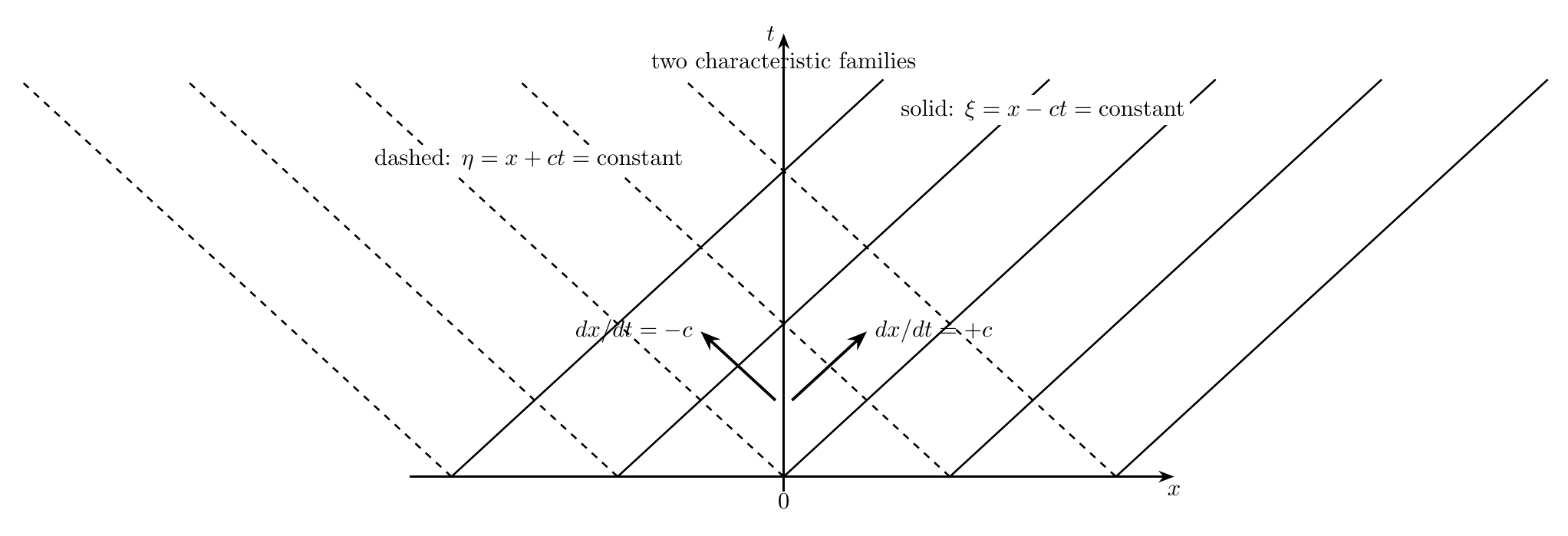
Figure. The two families of characteristic lines in the x-t plane. Solid lines carry constant ξ = x − ct and move toward increasing x; dashed lines carry constant η = x + ct and move toward decreasing x.

These lines are called characteristics. They organize how information propagates through the solution.

5 Rewrite the wave equation in characteristic coordinates

Let

u (x,t) = U (ξ,η).

(28)

Since

ξx = 1, ηx = 1,

(29)

we obtain

ux = U ξ + U η.

(30)

Differentiating again,

uxx = U ξξ + 2U ξη + U ηη.

(31)

Similarly,

ξ = − c, η = +c, t t

(32)

ut = − cUξ + cUη.

(33)

Differentiating again,

2 2 2 utt = c Uξξ − 2c Uξη + c Uηη.

(34)

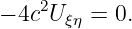
Therefore

u_tt − c²u_xx	= c²U_ξξ − 2c²U_ξη + c²U_ηη	(35)
	− c²	(36)
	= −4c²U_ξη.	(37)

The wave equation therefore becomes

− 4c2U = 0. ξη

(38)

For c≠0,

|--------| -Uξη =-0.-

(39)

This is much simpler than the original PDE.

6 Integrate the transformed equation

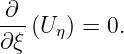
The equation

Uξη = 0

(40)

means

∂-- ∂ξ (Uη) = 0.

(41)

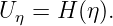
Therefore U_η cannot depend on ξ. It can depend only on η:

U η = H (η ).

(42)

Integrating with respect to η gives

U (ξ,η) = G (η) + F(ξ),

(43)

where the “constant of integration” with respect to η may still be an arbitrary function of ξ.

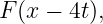
Returning to x and t,

|--------------------------------| |u(x,t) = F (x − ct) + G (x + ct). ---------------------------------

(44)

Thus, on a suitable domain and for sufficiently smooth functions, the general solution of the homogeneous one-dimensional constant-speed wave equation is the sum of one right-moving profile and one left-moving profile [4, 6].

7 What “general solution” means here

The statement

u (x,t) = F (x − ct) + G(x + ct)

(45)

is stronger than the verification result in WM15.

WM15 showed:

|------------------------------------------------------------| |if u = F (x − ct) or u = G (x + ct), then the PDE is satisfied. | -------------------------------------------------------------

(46)

WM16 shows, under the usual smoothness assumptions for a classical solution,

|-----------------------------------------------------------------------| every-solution-can-be-represented-locally-by-a-sum-of-these-two-families.--

(47)

The arbitrary functions F and G have not yet been determined. That requires initial or boundary data.

This distinction is essential:

|--------------------------------------------------------------------| |PDE structure tells us the form; data choose the particular solution. | ---------------------------------------------------------------------

(48)

8 The physical displacement is the sum of the two components

Suppose

uR(x,t) = F (x − ct)

(49)

and

uL (x,t) = G (x + ct).

(50)

Then the physical field is

u(x,t) = uR (x,t) + uL (x,t).

(51)

The addition is point by point.

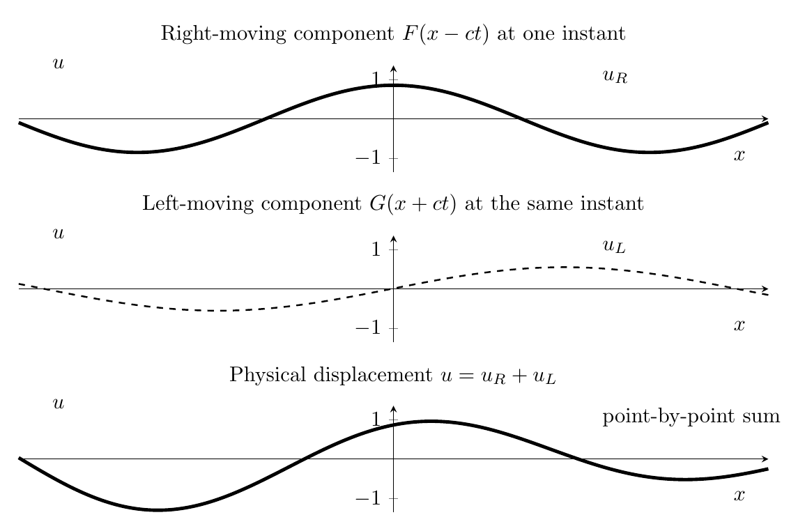
Figure. At any fixed time, the observed displacement is the point-by-point sum of a right-moving component and a left-moving component. Linearity allows both components to coexist without changing the governing equation.

Because the wave equation is linear, the two components propagate independently in the ideal model even while their sum may display interference.

9 Standing waves fit naturally into the two-family picture

Take equal-amplitude sinusoidal components

u_R(x,t)	= A cos(kx − ωt),	(52)
u_L(x,t)	= A cos(kx + ωt).	(53)

For the ideal wave equation,

ω = ck.

(54)

Adding the two components gives

u(x,t)	= A cos(kx − ωt) + A cos(kx + ωt)	(55)
	= 2A cos(kx) cos(ωt).	(56)

Therefore the Standing Waves studied earlier are not a separate species of solution. They are a particular superposition of equal right- and left-moving components.

This connects the standing-wave material of WM10 directly to the two-family structure of the wave equation.

10 A compact structural map

Figure. The logical chain from the second-order wave equation to its right- and left-moving solution families. WM17 will determine the two arbitrary functions from initial data.

11 Worked example 1: identify both traveling components

Consider

[ ] [ ] u(x, t) = exp − (x − 4t)2 + 1-exp − (x + 4t − 2)2 . 2

(57)

Identify the direction and speed of each component and state the wave equation it satisfies.

The first term is

F(x − 4t),

(58)

so it moves toward increasing x at speed

|------| |4m/s . -------

(59)

The second term can be written as

G(x + 4t),

(60)

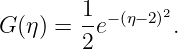
where

1-− (η−2)2 G (η) = 2e .

(61)

Therefore it moves toward decreasing x at the same speed magnitude,

|------| -4m/s--.

(62)

Because each term separately satisfies the wave equation and the equation is linear, their sum satisfies

|------------| -utt =-16uxx.|

(63)

12 Worked example 2: a non-obvious solution written as two traveling pieces

Consider

u(x,t) = xt.

(64)

Since

utt = 0

(65)

and

uxx = 0,

(66)

this function satisfies

2 utt = c uxx

(67)

for any constant c.

Can it really be written in right- and left-moving form?

Use the identity

(x + ct)2 − (x − ct)2 = 4cxt.

(68)

Therefore

(x + ct)2 (x − ct)2 xt = ---------− ---------. 4c 4c

(69)

Define

2 G (η) = η-- 4c

(70)

and

2 F (ξ) = − ξ-. 4c

(71)

Then

----------------------------- | | -xt-=-F-(x-−-ct) +-G-(x-+-ct).

(72)

This example shows that the two-family representation applies to more than localized pulses and sinusoids.

13 Worked example 3: decompose a standing wave

Suppose

u (x,t) = 6.0 mm cos(3x)cos(12t),

(73)

with x in meters and t in seconds.

Use

2 cosα cosβ = cos(α − β) + cos(α + β).

(74)

Then

u(x,t)	= 3.0 mm cos(3x − 12t)	(75)
	+ 3.0 mm cos(3x + 12t).	(76)

Hence the standing wave is the sum of

|--------------------------| -uR-=-3.0mm---cos(3x-−--12t)-

(77)

and

|--------------------------| uL = 3.0mm cos(3x + 12t).| ----------------------------

(78)

The common wave speed is

|--------| c = ω-= 12-= |4.0m/s . k 3 ---------

(79)

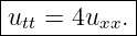
14 Worked example 4: verify a general two-family expression

Consider

u(x, t) = (x − 2t)3 + 2(x + 2t)2.

(80)

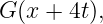
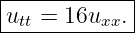
The first term is a function of x− 2t only, and the second is a function of x + 2t only. Therefore, by the WM15 result, each separately satisfies

utt = 4uxx.

(81)

Linearity then implies that the sum also satisfies

|----------| utt-=-4uxx.-

(82)

A direct check gives the same result.

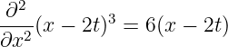
For the first term,

2 ∂--- 3 ∂x2(x − 2t) = 6(x − 2t)

(83)

and

∂2-- 3 ∂t2(x − 2t) = 24(x − 2t).

(84)

For the second term,

∂2 [ ] --2- 2(x + 2t)2 = 4 ∂x

(85)

and

∂2 [ ] --2- 2(x + 2t)2 = 16. ∂t

(86)

Thus

utt = 24(x − 2t) + 16

(87)

while

4uxx = 4 [6(x − 2t) + 4] = 24(x − 2t) + 16.

(88)

Therefore the PDE is satisfied everywhere.

15 Worked example 5: infer speed from the first-order relation

At one point in a known pure one-way wave, measurements give

ut = − 0.24m/s

(89)

and

ux = 0.0030.

(90)

Suppose the wave is known to be purely right-moving. Then

ut = − cux.

(91)

Hence

c	= −	(92)
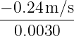	= −	(93)
	= 80 m/s .	(94)

The sign relation is consistent with rightward propagation because u_t and u_x have opposite signs.

This diagnostic is valid only when the field is known to contain a single traveling family. If both F and G are present simultaneously, the local ratio −u_t∕u_x generally does not equal c.

16 Worked example 6: connect the two-family solution to string mechanics

A stretched string has Tension

T = 180 N

(95)

and linear mass density

μ = 0.020 kg/m.

(96)

The string wave speed is

c	=	(97)
	=	(98)
	=	(99)
	≈ 94.9 m/s .	(100)

Suppose a sinusoidal component has

k = 6.0 rad/m.

(101)

Then

ω = ck

(102)

gives

ω	= (94.9)(6.0)	(103)
	≈ 569 rad/s .	(104)

A possible pair of equal-amplitude traveling components is therefore

|----------------------| |uR = A cos(6x − 569t )| ------------------------

(105)

and

|----------------------| |uL = A cos(6x + 569t).| ------------------------

(106)

Both components satisfy the same mechanically derived string equation

T- utt = μ uxx.

(107)

17 Common mistakes

Mistake: thinking x − ct means left-moving because of the minus sign. Holding the argument constant gives x = ct + constant, so the feature moves toward +x.
Mistake: applying u_t = −cu_x to a field containing both right- and left-moving components. That first-order equation applies to a pure right-moving component.
Mistake: treating the factorization of the wave operator as ordinary scalar multiplication without remembering that the factors are differential operators.
Mistake: concluding that a solution must look like a pulse or sinusoid. The arbitrary functions F and G can have many sufficiently smooth shapes.
Mistake: assuming the two functions F and G are known once the PDE is written. Initial or boundary data are needed to determine them.
Mistake: forgetting the smoothness assumptions behind the classical derivative manipulations.

18 What WM16 establishes

The one-dimensional constant-speed wave equation

utt = c2uxx

(108)

contains two characteristic propagation families:

|----------| |F (x − ct) | -----------

(109)

and

|----------| |G(x + ct).| ------------

(110)

For a sufficiently smooth classical solution on a suitable domain,

|--------------------------------| |u(x,t) = F (x − ct) + G (x + ct). ---------------------------------

(111)

The two components propagate in opposite directions at the same speed magnitude c.

The next problem is not to discover the form of the solution, but to determine the two arbitrary functions from physical data. That is the purpose of WM17: initial conditions and the d’Alembert solution.

References

[1] A. P. French, Vibrations and Waves, M.I.T. Introductory Physics Series, W. W. Norton & Company, 1971.

[2] Frank S. Crawford, Jr., Waves, Berkeley Physics Course, Volume 3, McGraw-Hill, 1968.

[3] William Moebs, Samuel J. Ling, and Jeff Sanny, University Physics, Volume 1, OpenStax, 2016, Section 16.2, “Mathematics of Waves.”

[4] Richard P. Feynman, Robert B. Leighton, and Matthew Sands, The Feynman Lectures on Physics, Volume I, Chapter 47, “Sound. The Wave Equation.”

[5] Richard P. Feynman, Robert B. Leighton, and Matthew Sands, The Feynman Lectures on Physics, Volume I, Chapter 48, “Beats.”

[6] Massachusetts Institute of Technology, 8.03SC Physics III: Vibrations and Waves, Lecture 10, “Traveling Waves,” MIT OpenCourseWare.

"Wave Mechanics: Right- and Left-Traveling Solutions" is owned by bloftin.
(view preamble)