Time Along the Orbit: Eccentric Anomaly, Mean Anomaly, and Kepler's Equation

1 The missing ingredient: time along a known ellipse

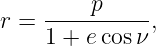
GPSORB04 showed that the ideal two-body orbit satisfies

-----p---- r = 1 + e cosν ,

(1)

and GPSORB05 showed how the instantaneous Cartesian state (r,v) determines the classical elements

(a,e,i,Ω, ω,ν).

(2)

The geometry is now well defined, but a propagation problem remains. Suppose a, e, i, Ω, and ω are known at some reference epoch. To predict the satellite position at a later time, one must determine how the in-plane phase evolves.

The most obvious candidate is true anomaly ν, because it is literally the angle at the occupied focus from periapsis to the radius vector. However, ν is not linear in time. From angular-momentum conservation,

h = r2˙ν,

(3)

-h ˙ν = r2 .

(4)

Because r changes around an eccentric orbit, the true-anomaly rate changes too. Near periapsis r is small and the true-anomaly rate is large; near apoapsis r is large and the rate is small.

The goal of this article is therefore to introduce an angular variable that is easy to connect to geometry, and then another angular variable that advances uniformly in time.

2 The auxiliary circle and eccentric anomaly

Consider an ellipse with semimajor axis a and semiminor axis

√ ------ b = a 1 − e2.

(5)

Place the occupied focus at the origin. The ellipse center is then displaced by ae from the focus along the major axis. With periapsis on the positive x axis, the center lies at

x = − ae. c

(6)

Construct an auxiliary circle of radius a centered on the ellipse center. For a point on the ellipse, extend a vertical line to the auxiliary circle. The angle from the positive major-axis direction to the radius of the auxiliary circle is called the eccentric anomaly E.

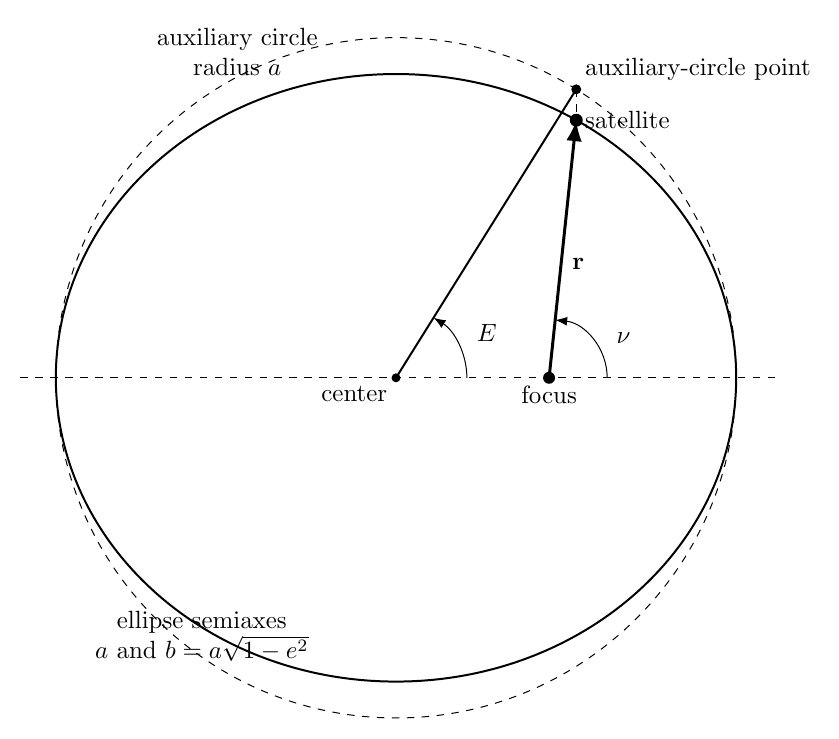
Figure 1. Eccentric anomaly is measured at the ellipse center on an auxiliary circle, while true anomaly is measured at the focus.

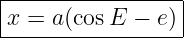
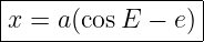
This construction immediately gives the focus-centered coordinates of the satellite. The auxiliary-circle point has horizontal coordinate

x = − ae + a cosE.

(7)

The ellipse compresses the vertical coordinate by the factor b∕a, so

y = b sin E.

(8)

Using Eq. (5),

|----------------| |x = a(cosE − e)| ------------------

(9)

and

|--------------------| | √ -----2 | -y-=-a--1-−-e--sin-E.-

(10)

These equations are fundamental because they connect the ellipse geometry to the parameter E.

3 Orbital radius expressed through eccentric anomaly

The focus-centered orbital radius is

∘ -------- r = x2 + y2.

(11)

Substitute Eqs. (9) and (10):

r2 = a2(cosE − e)2 + a2(1 − e2)sin2E.

(12)

Factor out a²:

2 r--= (cosE − e)2 + (1 − e2)sin2E. a2

(13)

Expand:

r2 2 2 2 2 2 --2 = cos E − 2ecosE + e + sin E − e sin E. a

(14)

Since cos ²E + sin ²E = 1,

2 r--= 1 − 2ecos E + e2cos2 E. a2

(15)

The right side is a perfect square:

r2 -2-= (1 − e cosE )2. a

(16)

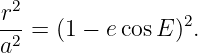
For an ellipse r > 0, so

|------------------| |r = a(1 − ecosE ).| --------------------

(17)

This result gives useful checks. At periapsis, E = 0 and

rp = a(1 − e).

(18)

At apoapsis, E = π and

ra = a(1 + e).

(19)

4 Swept area from the eccentric-anomaly parametrization

Kepler’s second law says that the radius vector sweeps equal areas in equal times. GPSORB03 derived

|--------| | ˙ h- | |A = 2 .| ---------

(20)

To connect this time law to eccentric anomaly, compute the area swept from periapsis to the current point.

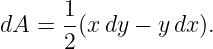
For any planar curve parameterized by x(E) and y(E), the differential area swept about the origin is

dA = 1-(xdy − y dx). 2

(21)

From Eqs. (9) and (10),

dx = − a sin E dE,

(22)

and

dy = bcos E dE.

(23)

Therefore

x dy − y dx = a(cos E − e)bcos E dE + absin2E dE.

(24)

Factor ab:

( ) x dy − y dx = ab cos2E − ecosE + sin2 E dE.

(25)

Hence

xdy − ydx = ab(1 − e cosE )dE.

(26)

Substitute this into Eq. (21):

dA = ab(1 − ecosE )dE. 2

(27)

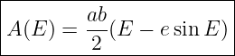
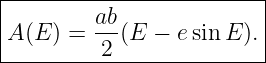
Integrating from periapsis, where E = 0, to the current eccentric anomaly E gives

∫ ab E A(E ) = --- (1 − e cosu) du. 2 0

(28)

Therefore

|------------------------| | ab- | |A(E ) = 2 (E − esinE ).| --------------------------

(29)

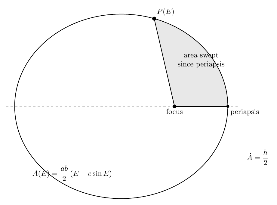
Figure 2. The swept area from periapsis can be written directly in terms of eccentric anomaly.

Equation (29) is the geometric origin of Kepler’s equation.

5 Orbital period from the area law

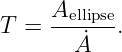
The total area of the ellipse is

A = πab. ellipse

(30)

Because the area sweep rate is constant,

Aellipse T = ---˙--. A

(31)

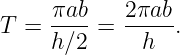
Using Eq. (20),

T = πab-= 2πab-. h∕2 h

(32)

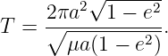
GPSORB04 derived

2 h = μp

(33)

with

p = a(1 − e2).

(34)

Thus

∘ ----------- h = μa(1 − e2).

(35)

Also,

------ b = a√ 1 − e2.

(36)

Substitute both expressions into Eq. (32):

2 πa2√1--−-e2 T = ∘------------. μa(1 − e2)

(37)

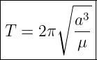
The eccentricity factors cancel, leaving

|------∘-----| | a3 | T = 2π μ-.| --------------

(38)

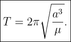
This is Kepler’s third law in two-body form.

A striking feature is that for a fixed central body the period depends only on the semimajor axis, not on eccentricity.

6 Mean motion

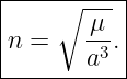
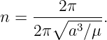
Define the mean motion as the uniform angular rate corresponding to one complete revolution in one orbital period:

2π n ≡ ---. T

(39)

Using Eq. (38),

n = --∘2π----. 2π a3∕μ

(40)

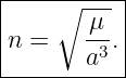
Therefore

|----------| | ∘ -μ- | |n = --.| --------a3--

(41)

The units are radians per second if radians are retained as the angular unit.

Mean motion is not the instantaneous true-anomaly rate. In general,

n ⁄= ˙ν.

(42)

The quantity n is a constant for the ideal Kepler ellipse because a is constant.

7 Mean anomaly

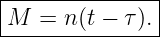
Let τ denote the time of periapsis passage. Define the mean anomaly

|--------------| |M = n(t − τ).| ----------------

(43)

By construction, M increases uniformly from 0 to 2π during one orbital period.

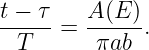
The fraction of an orbital period elapsed since periapsis is

t −-τ-. T

(44)

Because area is swept uniformly in time, the same fraction equals the swept-area fraction:

t −-τ A-(E-)- T = πab .

(45)

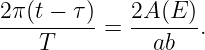
Multiply by 2π:

2π(t-−-τ)-= 2A-(E-). T ab

(46)

The left side is mean anomaly because n = 2π∕T:

M = 2A-(E). ab

(47)

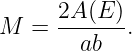
Now substitute Eq. (29):

[ ] 2 ab M = ab- 2-(E − esinE ) .

(48)

Thus

|------------------| -M--=--E-−-e-sin-E.-|

(49)

This is Kepler’s equation for an elliptic orbit.

The equation is conceptually simple but mathematically important: time determines M linearly, but the geometry of the ellipse makes the conversion from M to E nonlinear.

8 Propagation from a reference epoch

In practical navigation work, one usually propagates from a reference epoch t₀ rather than from the most recent periapsis passage. Let the mean anomaly at the reference epoch be M₀. Then

M0 = n(t0 − τ).

(50)

At a later time,

M = n(t − τ).

(51)

Subtract the two equations:

M − M0 = n(t − t0).

(52)

Hence

|-----------------------| M (t) = M + n(t − t ). | ----------0----------0---

(53)

This is why mean anomaly is so useful in ephemeris propagation: the difficult orbital speed variation has been moved into the nonlinear transformation from M to E.

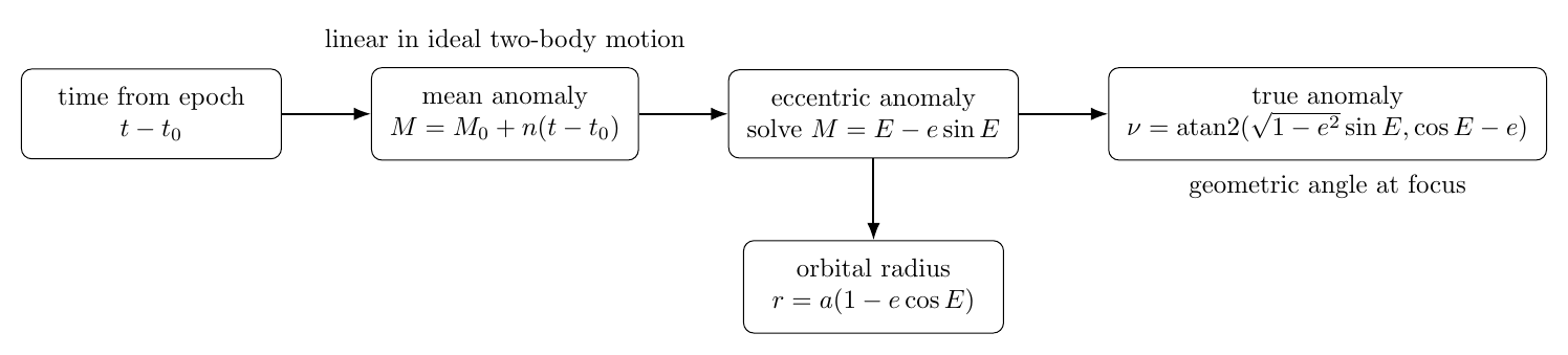
Figure 3. Time propagation proceeds linearly in mean anomaly, then nonlinearly through eccentric anomaly to true anomaly and radius.

9 Why Kepler’s equation must be solved

Given time, Eq. (53) provides M. Kepler’s equation then requires

M = E − e sin E.

(54)

The unknown E appears both by itself and inside a sine function. There is no finite combination of ordinary algebraic and elementary transcendental operations that isolates E in the same way one solves a linear or quadratic equation. In navigation software, E is therefore normally obtained by iteration.

Define

f (E) = E − esinE − M.

(55)

The desired eccentric anomaly satisfies

f(E ) = 0.

(56)

Its derivative is

′ f (E) = 1 − e cosE.

(57)

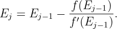
Newton’s method gives

Ej = Ej− 1 − f(Ej-−1). f′(Ej −1)

(58)

Therefore

|------------------------------------| | M--−-Ej−-1 +-e-sin-Ej−-1| |Ej = Ej −1 + 1 − ecos E .| ----------------------------j−1------

(59)

For the small eccentricities typical of GPS orbits, E₀ = M is an excellent initial guess.

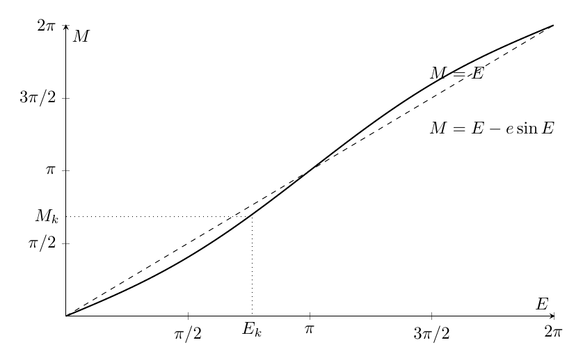
Figure 4. Kepler’s equation maps a known mean anomaly to the eccentric anomaly that must be solved for.

10 From eccentric anomaly to true anomaly

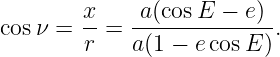
The same satellite point can be described either by eccentric anomaly E or true anomaly ν. Because the focus is the origin,

x = rcos ν, y = r sin ν.

(60)

Using Eqs. (9), (10), and (17),

cos ν = x-= -a(cosE-−--e). r a(1 − ecos E)

(61)

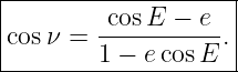
Therefore

|--------------------| | cosE − e | |cosν = -----------.| ---------1 −-ecos-E--

(62)

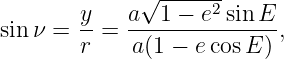
Similarly,

√ ------ sin ν = y-= a--1-−-e2-sin-E-, r a(1 − ecosE )

(63)

|-------√------2-------| |sin ν = --1-−-e--sin-E-.| ----------1 −-ecosE----|

(64)

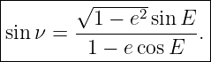
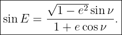
The denominator is common to both sine and cosine and is positive for an ellipse. Therefore a quadrant-safe expression is

|---------(------------------------)--| | √ ----2- | ν-=-atan2-----1 −-e-sin-E,-cosE-−--e-.--

(65)

If a software implementation returns angles in (−π,π] and an angle in [0, 2π) is desired, add 2π when the result is negative.

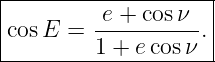
11 From true anomaly back to eccentric anomaly

The inverse transformation follows from the same geometry. Starting with Eq. (62), solve for cos E:

cosν(1 − e cosE ) = cosE − e.

(66)

Collect the cos E terms:

cos ν + e = cosE (1 + ecosν ).

(67)

Hence

|--------------------| |cosE = -e-+-cosν- .| ---------1-+-e-cosν--|

(68)

A similar manipulation gives

|----------------------| | √1--−-e2sinν | |sin E = -------------.| ----------1-+-e-cosν---

(69)

The common denominator is again positive for an ellipse, so the inverse quadrant-safe form is

|----------(----------------------)--| |E = atan2 √1 − e2 sin ν,e + cosν .| --------------------------------------

(70)

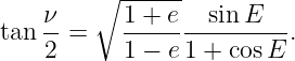
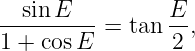
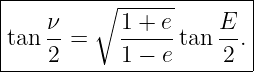
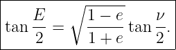
12 Half-angle relations

Many orbital-mechanics texts express the relationship between E and ν with half-angle identities. Begin with

ν sinν tan-- = ---------. 2 1 + cosν

(71)

Substitute Eqs. (64) and (62). The common denominator 1 − e cos E cancels:

√ ------ ν- -------1 −-e2sinE------ tan 2 = 1 − e cosE + cosE − e.

(72)

The denominator factors as

1 − ecos E + cos E − e = (1 − e)(1 + cosE ).

(73)

Since

√ ------ ∘ -------------- 1 − e2 = (1 − e)(1 + e),

(74)

we obtain

∘ ------ ν- 1-+-e --sin-E---- tan 2 = 1 − e 1 + cosE .

(75)

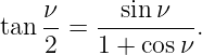
Using

sin E E ----------= tan --, 1 + cos E 2

(76)

we arrive at

|-------∘---------------| | ν- 1-+-e E- | tan 2 = 1 − e tan 2 .| -------------------------

(77)

The inverse relation is

|--------∘--------------| | E- 1 −-e ν- | tan 2 = 1 + e tan 2.| -------------------------

(78)

The half-angle formulas are compact, but a direct one-argument inverse tangent can lose quadrant information. For robust numerical work, Eqs. (65) and (70) are generally preferable.

13 Mean anomaly is not a physical line in the ellipse

It is important not to confuse the three anomalies.

Quantity	Where the angle is associated	Physical role
True anomaly ν	occupied focus	actual geometric direction of the radius vector from periapsis
Eccentric anomaly E	ellipse center and auxiliary circle	geometric parameter that makes the ellipse algebraically simple
Mean anomaly M	uniform phase variable	time-like angle that increases linearly at rate n

True anomaly and eccentric anomaly have direct geometric constructions. Mean anomaly is primarily a time coordinate. One can visualize it as the angle of a fictitious body moving uniformly around a reference circle, but in the actual ellipse it should be understood through

M = n (t − τ)

(79)

and

M = E − e sin E.

(80)

14 A useful differential relation

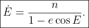
Differentiate Kepler’s equation with respect to time:

M˙ = E˙ − ecos E E˙.

(81)

For ideal Keplerian motion,

M˙ = n.

(82)

Therefore

n = E˙(1 − ecos E ).

(83)

Hence

|----------------| E˙ = -----n-----.| -----1-−-e-cosE---

(84)

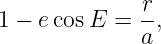
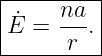
Using Eq. (17),

1 − ecosE = -r, a

(85)

|----na--| E˙ = ---.| ------r---

(86)

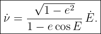
This rate is not constant. Eccentric anomaly is easier than true anomaly geometrically, but only mean anomaly advances uniformly.

Differentiating the E-to-ν transformation gives the useful result

|-----√------------| | 1 − e2 | |˙ν = -----------E˙. | -----1-−-ecos-E-----

(87)

Combining Eqs. (84) and (87) provides a direct route to the true-anomaly rate used later in velocity derivations.

15 Worked GPS-like numerical example

Consider an idealized GPS-like ellipse with

a = 26560 km, e = 0.01,

(88)

and use

μ = 398600.5 km3 ∕s2.

(89)

Assume the satellite passed periapsis at t = 0 and evaluate its orbital phase two hours later:

t = 7200 s.

(90)

First compute the mean motion:

∘ --------- n = 398600.5-≈ 1.458568 × 10− 4 rad/s. 265603

(91)

The corresponding orbital period is

2π- T = n ≈ 43077.8 s ≈ 11.966 h.

(92)

Because periapsis occurred at t = 0,

M = nt.

(93)

Thus

M ≈ 1.050169 rad ≈ 60.1703∘.

(94)

Now solve

E − 0.01 sin E = M.

(95)

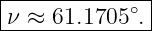
Newton iteration with E₀ = M converges rapidly to

∘ E ≈ 1.058887 rad ≈ 60.6698 .

(96)

Use the quadrant-safe transformation:

( √ --------- ) ν = atan2 1 − 0.012 sin E, cosE − 0.01 .

(97)

This gives

|--------------| -ν-≈-61.1705-∘.|

(98)

Finally,

r = a(1 − ecosE ),

(99)

|----------------| |r ≈ 26429.9 km. | ------------------

(100)

The three angles are close because e = 0.01 is small, but they are not identical:

∘ ∘ ∘ M ≈ 60.17 , E ≈ 60.67 , ν ≈ 61.17 .

(101)

16 Circular-orbit limit

If e = 0, the ellipse becomes a circle. Then

r = a,

(102)

and Kepler’s equation becomes

M = E.

(103)

Equations (62) and (64) reduce to

cosν = cosE, sinν = sin E.

(104)

Therefore, modulo 2π,

|------------| -M--=-E--=-ν-|

(105)

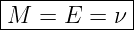
for the ideal circular case.

This limit is a valuable sanity check: all three anomaly variables collapse to the same uniformly advancing angle.

17 Connection to the GPS broadcast navigation equations

The first part of the legacy GPS broadcast ephemeris algorithm follows almost exactly the chain derived here. The navigation message supplies √ --
A , e, a reference epoch t_oe, a mean anomaly at epoch M₀, and a mean-motion correction Δn.

The user first reconstructs the semimajor axis,

√ -- 2 A = ( A ) ,

(106)

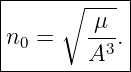
then computes the nominal Keplerian mean motion,

|-----∘------| | μ-- | |n0 = A3 .| -------------

(107)

The broadcast model modifies that ideal rate through

n = n0 + Δn.

(108)

For

tk = t − toe,

(109)

mean anomaly is propagated as

|----------------| |Mk = M0 + ntk.| ------------------

(110)

Then Kepler’s equation is solved,

|--------------------| |M = E − esin E ,| ---k-----k---------k-

(111)

and the resulting E_k is converted to true anomaly ν_k.

Thus the first several lines of the GPS user algorithm are not an arbitrary sequence of navigation-message formulas. They are the direct engineering implementation of the two-body time propagation developed in this article, with Δn added because the operational broadcast orbit is a fitted, perturbed model rather than an exact Kepler ellipse.

The GPS interface specification also requires the time difference t_k to be adjusted across GPS-week boundaries when necessary. That bookkeeping belongs to the operational time system, not to the underlying Kepler derivation, but it is essential in receiver software.

18 Summary

Eccentric anomaly provides a convenient parameterization of an ellipse:

|----------------| -x =-a(cosE--−-e)-

(112)

and

|-----√------2------| -y-=-a--1-−-e--sin-E-.

(113)

From these coordinates follows

|------------------| -r =-a(1 −-ecosE-)-.

(114)

Combining the eccentric-anomaly parameterization with the constant area-sweep law gives

|------------------------| | ab | |A (E ) = -2-(E − e sin E) | -------------------------

(115)

and therefore Kepler’s equation

|------------------| -M--=--E-−-e-sin-E.-|

(116)

The orbital period and mean motion are

|-------∘----| | 3 | |T = 2π a--| | μ | --------------

(117)

and

|----∘-----| | μ--| |n = a3.| ------------

(118)

Mean anomaly therefore propagates linearly:

|--------------------| M---=-M0-+--n(t −-t0).-

(119)

The robust eccentric-anomaly to true-anomaly transformation is

|---------(------------------------)--| | √ ----2- | ν-=-atan2-----1 −-e-sin-E,-cosE-−--e-,--

(120)

and the inverse is

|----------(-√--------------------)--| |E = atan2 1 − e2 sin ν,e + cosν .| --------------------------------------

(121)

The complete ideal propagation chain is therefore

|----------------------------| -t −-→-M--−→--E-−-→--ν-−→--r.|

(122)

This is the mathematical core of the time-propagation portion of the GPS broadcast ephemeris.

References

[1] E. D. Kaplan and C. J. Hegarty, eds., Understanding GPS/GNSS: Principles and Applications, 3rd ed., Artech House, 2017.

[2] R. R. Bate, D. D. Mueller, and J. E. White, Fundamentals of Astrodynamics, Dover Publications, 1971.

[3] D. A. Vallado, Fundamentals of Astrodynamics and Applications, 4th ed., Microcosm Press, 2013.

[4] H. D. Curtis, Orbital Mechanics for Engineering Students, 4th ed., Elsevier, 2020.

[5] Global Positioning Systems Directorate, IS-GPS-200N: NAVSTAR GPS Space Segment/Navigation User Interfaces, 1 August 2022, Table 20-IV. https://www.gps.gov/technical/icwg/IS-GPS-200N.pdf

"Time Along the Orbit: Eccentric Anomaly, Mean Anomaly, and Kepler's Equation" is owned by bloftin.
(view preamble)