1 From six Cartesian coordinates to six geometric coordinates
The inertial Cartesian state is
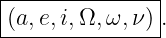
It contains six independent scalars. For ideal two-body motion, the same physical state may be
represented by
The two descriptions answer different questions. Cartesian coordinates say where the satellite is
and how fast it is moving in a chosen frame. The classical orbital elements separate the same
information into orbit size, orbit shape, plane orientation, orientation within the plane, and current
phase.
A useful interpretation is
| Element | Geometric role |
| a | orbit size and energy |
| e | orbit shape |
| i | tilt of the orbital plane |
| Ω | orientation of the line of nodes in the reference plane |
| ω | direction of periapsis within the orbital plane |
| ν | current satellite location measured from periapsis |
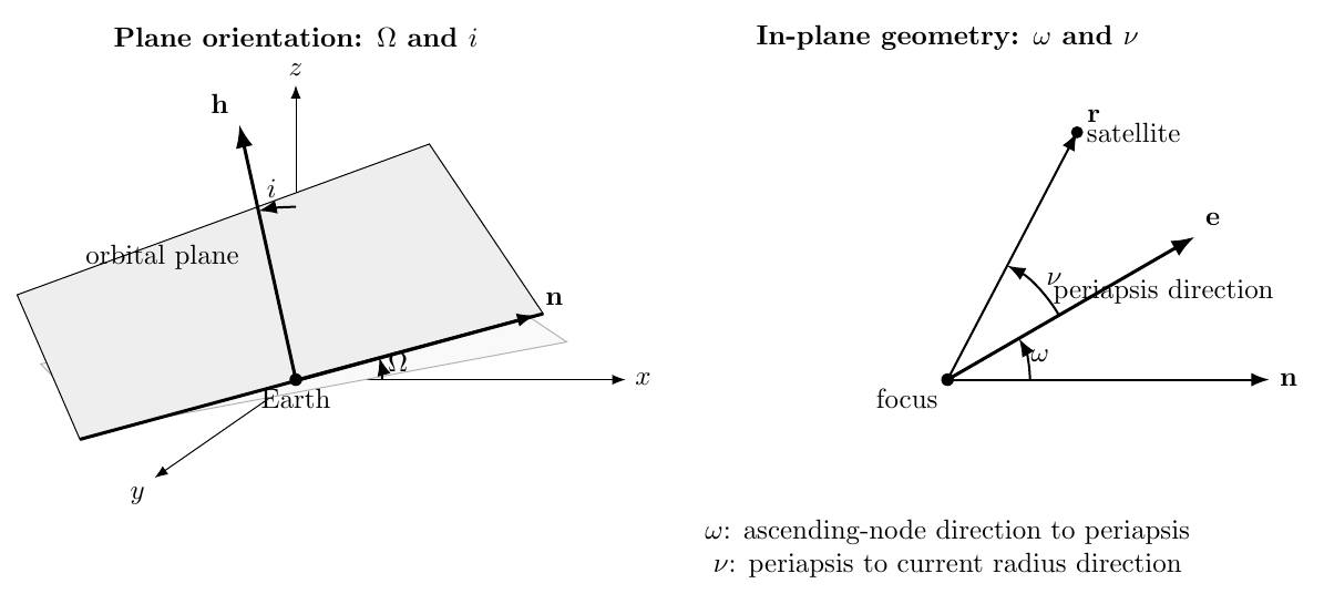
Figure 1. The classical angles divide naturally into plane-orientation angles and in-plane angles.
GPSORB02 established the need for six constants. GPSORB03 derived angular momentum.
GPSORB04 derived mechanical energy and eccentricity. These quantities now yield the classical
orbital elements.
2 Required auxiliary quantities
Given r and v, begin with their magnitudes
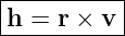
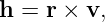
The specific angular-momentum vector is
with magnitude
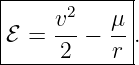
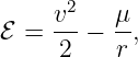
The specific mechanical energy is
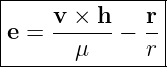
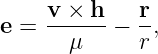
The eccentricity vector is
and its magnitude is
The inertial reference plane is assumed to be the x-y plane, with unit normal
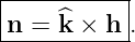
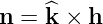
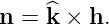
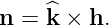
The node vector is defined by
Because n lies in both the inertial reference plane and the orbital plane, it points along their
intersection: the line of nodes. For the usual prograde geometry, n points toward the ascending
node.
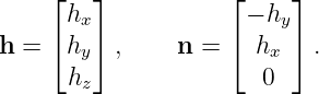
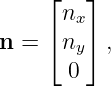
In components,
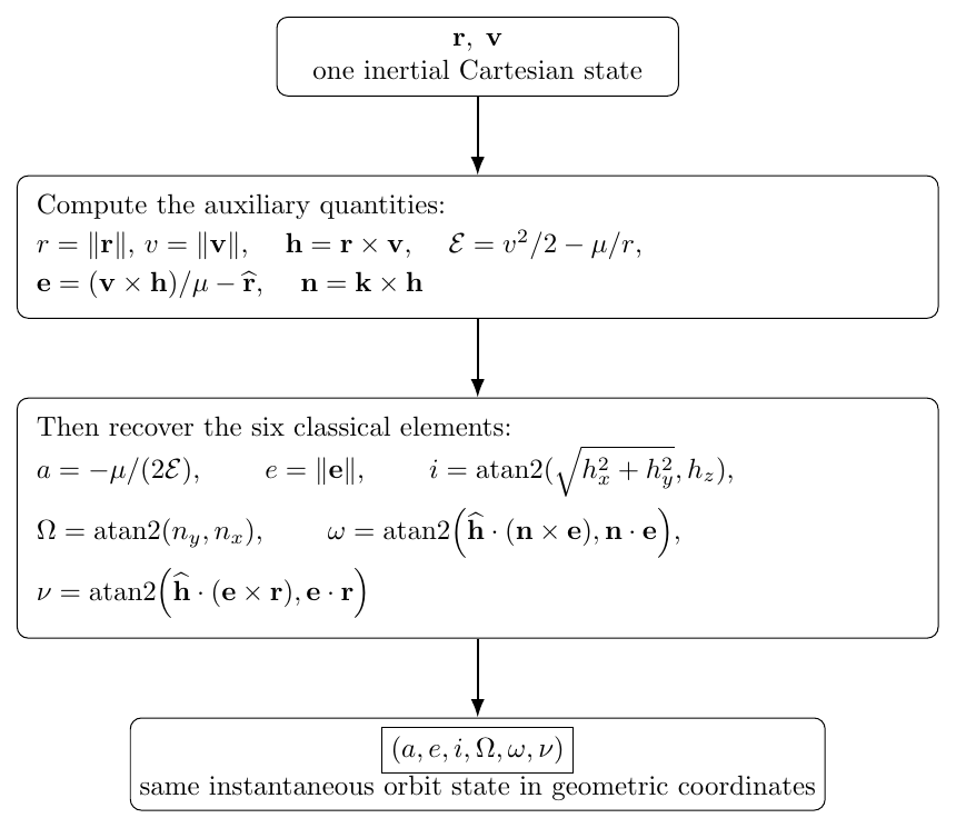
Figure 2. Practical computation chain from one inertial Cartesian state to the six classical
elements.
3 Semimajor axis from the specific mechanical energy
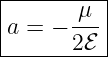
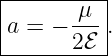
GPSORB04 derived
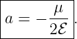
for a nonparabolic Kepler orbit. Therefore
For an ellipse, ℰ < 0 and therefore a > 0. For a hyperbola, ℰ > 0 and the conventional semimajor
axis is negative. At the parabolic limit,
so |a|→∞. The semilatus rectum
remains finite and is often a better size parameter near the parabolic limit.
The first element therefore comes directly from energy: no angle extraction is required.
4 Eccentricity from the eccentricity vector
The second element is simply the magnitude of Eq. (7):
The magnitude determines the conic type,
The direction of e is equally important: for e≠0, it points toward periapsis. That direction will be
used to define ω and ν.
5 Why atan2 is preferable to inverse cosine
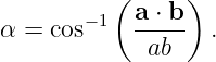
Many orbital-mechanics derivations introduce angles with formulas such as
This recovers an angle only in the interval 0 ≤ α ≤ π. The cosine does not tell us on which side of
the reference direction the target vector lies. A second sign test must therefore be added by
hand.
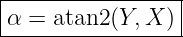
A more systematic method computes both a cosine-like and sine-like quantity and uses
where X is proportional to cos α and Y is proportional to sin α. The signs of both arguments
preserve the quadrant.
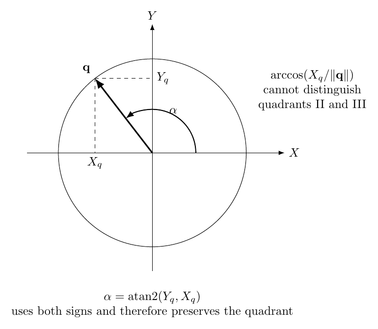
Figure 3. atan2 uses both component signs and therefore preserves quadrant information that
arccos alone loses.
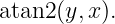
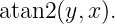
Most numerical libraries use the argument order
MATLAB, Python, C, C++, and many other environments follow this convention. The returned
interval is commonly (−π,π]. Orbital elements are often reported on [0, 2π), so a negative result
may be wrapped by adding 2π.
6 Inclination from the angular-momentum vector
The orbital plane is perpendicular to h. The reference x-y plane is perpendicular to k. Therefore
the inclination is the angle between h and k.
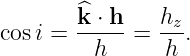
The usual cosine relation is
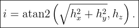
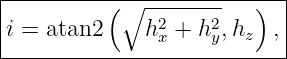
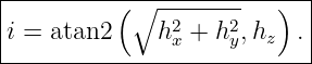
Instead of using only arccos, form the sine magnitude from
Then
This naturally returns
Thus prograde orbits satisfy 0 ≤ i < π∕2, polar orbits have i = π∕2, and retrograde orbits satisfy
π∕2 < i ≤ π.
7 Right ascension of the ascending node
The node vector
lies in the reference plane and points toward the ascending-node direction. Since
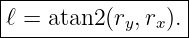
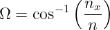
the right ascension of the ascending node is simply its polar angle measured from the positive
inertial x axis:
If the result is negative, wrap it to [0, 2π).
Using Eq. (11), one could equivalently write
but computing n explicitly makes the geometry clearer and is less error-prone.
The formula requires
When n = 0, the orbit is equatorial and there is no unique ascending node. That singular case is
treated later.
8 Argument of periapsis
The argument of periapsis is the oriented angle within the orbital plane from the ascending-node
direction n to the eccentricity vector e.
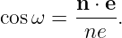
The cosine is
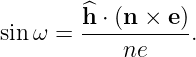
To obtain the sign of the sine, note that h is the positive normal to the orbital plane.
Therefore
Combining the two with atan2 gives
The common positive scale factor ne cancels between the two arguments, so normalization is
unnecessary inside the atan2 call.
This formula requires both
If the orbit is equatorial, the node direction disappears. If the orbit is circular, the periapsis
direction disappears.
9 True anomaly
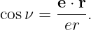
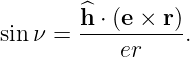
The true anomaly is the oriented angle from the eccentricity vector to the instantaneous radius
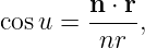
vector. Its cosine is
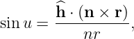
The corresponding signed sine is
Therefore
Again, the common scale factor er does not need to be included explicitly.
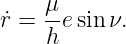
A useful cross-check follows from the radial-velocity result derived in GPSORB04,
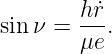
Hence, for e≠0,
This makes the physical sign intuitive: before apoapsis the satellite is moving outward and ṙ > 0;
after apoapsis it is moving inward and ṙ < 0.
10 The complete nonsingular state-to-elements algorithm
For a noncircular, nonequatorial orbit, the transformation can be written compactly as
follows.
First compute
and
Then
for a nonparabolic orbit,
and
Wrap Ω, ω, and ν into the desired 2π interval after the call to atan2.
11 A GPS-like numerical example
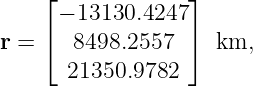
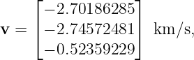
To make the full transformation concrete, consider the inertial state
with
The state was chosen to be representative of a medium-Earth orbit, but the conversion procedure
is completely general for a nondegenerate Kepler orbit.
The magnitudes are
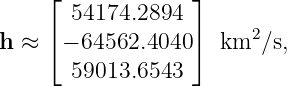
The angular-momentum vector is
with
The energy is
Therefore
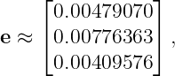
The eccentricity vector is
so
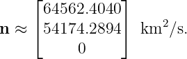
The node vector is
Applying the quadrant-safe formulas gives
and
Thus the recovered classical element set is
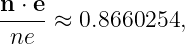
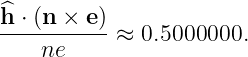
As a useful numerical check,
while
These are cos 30∘ and sin 30∘, respectively. Likewise, the true-anomaly formulas recover
approximately cos 70∘ and sin 70∘.
12 Why the classical elements become singular
The Cartesian state remains perfectly well defined for circular and equatorial orbits, but some of
the geometric reference directions used by the classical elements disappear. These are coordinate
singularities, not physical singularities.
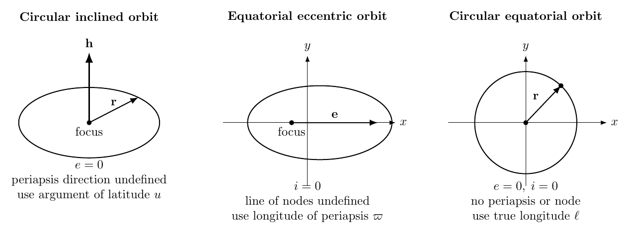
Figure 4. Classical-element singularities occur when periapsis or the line of nodes ceases to define
a unique direction.
12.1 Circular inclined orbit
For a circular orbit,
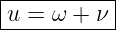
There is no unique periapsis direction, so ω and ν are individually undefined. Their sum, however,
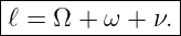
remains meaningful. Define the argument of latitude
where the symbol u is conventionally used. Directly from the state,
so
12.2 Equatorial eccentric orbit
For a prograde equatorial orbit,
so
There is no unique ascending node, and therefore Ω and ω are individually undefined. Their sum
remains meaningful as the longitude of periapsis,
For a prograde equatorial orbit it can be obtained directly from the eccentricity vector:
Retrograde equatorial motion requires careful sign conventions because the positive orbital normal
is opposite the reference z direction; modified or equinoctial elements are generally preferable near
that singular geometry.
12.3 Circular equatorial orbit
Now both the periapsis direction and node direction disappear. The four classical angles Ω, ω, and
ν do not remain individually meaningful, but the satellite’s azimuth in the reference plane does.
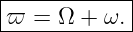
Define the true longitude
For a prograde circular equatorial orbit,
Again, the physical state is not singular. Only the chosen coordinates are.
13 Practical singularity thresholds
In floating-point software one should not test exact equality such as
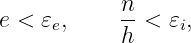
Instead choose tolerances appropriate to the application. A generic implementation might classify
the orbit using thresholds
where 𝜀e and 𝜀i are selected based on numerical precision and mission requirements.
This matters because the classical angles become poorly conditioned before the exact singularity is
reached. If e is extremely small, tiny state-vector perturbations can rotate the computed periapsis
direction dramatically even though the physical orbit has barely changed. Similarly, when i is
extremely small, tiny perturbations can move the computed node direction by a large
angle.
For estimation and orbit propagation, nonsingular element sets such as equinoctial or modified
equinoctial elements are often preferred near these geometries. The classical elements remain
extremely useful for interpretation because their geometry is intuitive.
14 Common implementation errors
Several mistakes recur in state-to-element software.
14.1 Reversing the cross product in the node vector
The adopted definition is
Using h ×k reverses the vector and shifts the node angle by π.
14.2 Using inverse cosine without a quadrant test
A formula such as
does not distinguish positive and negative ny. The atan2 form does.
14.3 Swapping the arguments of atan2
The convention used here is
Swapping those arguments changes the angle definition.
14.4 Forgetting angle wrapping
An atan2 result of −10∘ may represent the desired orbital angle 350∘. The mathematical direction
is the same, but software interfaces often require one specified interval.
14.5 Applying nonsingular formulas to singular geometry
If e or n is numerically near zero, formulas for ω, ν, or Ω may divide by tiny quantities or return
essentially arbitrary directions. The orbit must first be classified and the appropriate replacement
angle selected.
15 Connection to GPS broadcast ephemeris parameters
The classical element set derived here is not yet the full GPS broadcast model, but it explains the
geometry behind several broadcast parameters. The legacy GPS ephemeris contains quantities
corresponding closely to
plus rates and harmonic correction terms.
There is one important difference from the element set in Eq. (2): the navigation message uses
mean anomaly at the reference epoch rather than true anomaly as its phase variable. True anomaly
is geometrically natural for locating the satellite on the conic, while mean anomaly is much
more convenient for time propagation because it advances linearly in the ideal Kepler
problem.
The next lessons therefore move from the geometric angle ν to eccentric anomaly E and mean
anomaly M, derive Kepler’s equation, and show why the broadcast ephemeris begins its time
update with mean motion and mean anomaly.
16 Summary
One inertial Cartesian state
contains exactly the information required to reconstruct the six classical orbital elements.
Energy gives the orbit size,
The eccentricity vector gives the shape,
The angular-momentum vector gives the plane tilt,
The node vector gives the orientation of the orbital plane in inertial space,
The node and eccentricity vectors determine the periapsis orientation,
and the eccentricity and radius vectors determine the instantaneous position on the
conic,
The classical elements are therefore not an unrelated set of geometric labels. They are a nonlinear
change of coordinates on the same six-dimensional orbital state. Their circular and equatorial
singularities arise because some geometric reference directions cease to exist, not because the
satellite dynamics themselves become singular.
References
[1] E. D. Kaplan and C. J. Hegarty, eds., Understanding GPS/GNSS: Principles and
Applications, 3rd ed., Artech House, 2017.
[2] R. R. Bate, D. D. Mueller, and J. E. White, Fundamentals of Astrodynamics, Dover
Publications, 1971.
[3] D. A. Vallado, Fundamentals of Astrodynamics and Applications, 4th ed., Microcosm
Press, 2013.
[4] H. D. Curtis, Orbital Mechanics for Engineering Students, 4th ed., Elsevier, 2020.
[5] R. Broucke and P. Cefola, “On the Equinoctial Orbit Elements,” Celestial Mechanics,
vol. 5, pp. 303–310, 1972.

![[r] [ ]T
x = = x y z vx vy vz .
v](https://images.physicslibrary.org/cache/objects/1261/make4ht/ClassicalOrbitalElementsFromPositionAndVelocity0x.png)