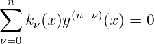
Let us consider the linear homogeneous differential equation
of order n. If the coefficient functions kν(x) are continuous and the coefficient k0(x) of the highest
order derivative does not vanish on a certain interval (resp. a domain in ℂ), then all solutions y(x)
are continuous on this interval (resp. domain). If all coefficients have the continuous derivatives up
to a certain order, the same concerns the solutions.
If, instead, k0(x) vanishes in a point x0, this point is in general a singular point. After dividing the
differential equation by k0(x) and then getting the form
some new coefficients cν(x) are discontinuous in the singular point. However, if the discontinuity is
restricted so, that the products
are continuous, and even analytic in x0, the point x0 is a regular singular point of the differential
equation.
We introduce the so-called Frobenius method for finding solution functions in a neighbourhood of
the regular singular point x0, confining us to the case of a second order differential equation. When
we use the quotient forms
where r(x), p(x) and q(x) are analytic in a neighbourhood of x0 and r(x)≠0, our differential
equation reads
| (x − x0)2r(x)y′′(x) + (x − x
0)p(x)y′(x) + q(x)y(x) = 0. | | (1) |
Since a simple change x−x0 x of variable brings to the case that the singular point is the origin,
we may suppose such a starting situation. Thus we can study the equation
x of variable brings to the case that the singular point is the origin,
we may suppose such a starting situation. Thus we can study the equation
| x2r(x)y′′(x) + xp(x)y′(x) + q(x)y(x) = 0, | | (2) |
where the coefficients have the converging power series expansions
| r(x) = ∑
n=0∞r
nxn, p(x) = ∑
n=0∞p
nxn, q(x) = ∑
n=0∞q
nxn | | (3) |
and
In the Frobenius method one examines whether the equation (2) allows a series solution of the
form
| y(x) = xs ∑
n=0∞a
nxn = a
0xs + a
1xs+1 + a
2xs+2 + …, | | (4) |
where s is a constant and a0≠0.
Substituting (3) and (4) to the differential equation (2) converts the left hand side to
| [r0s(s−1)+p0s+q0]a0xs+ | |
|
| [[r0(s+1)s+p0(s+1)+q0]a1+[r1s(s−1)+p1s+q1]a0]xs+1+ | |
|
| [[r0(s+2)(s+1)+p0(s+2)+q0]a2+[r1(s+1)s+p1(s+1)+q1]a1+[r2s(s−1)+p2s+q2]a0]xs+2+ … | | |
Our equation seems clearer when using the notations fν(s) := rνs(s−1) + pνs + qnu:
| f0(s)a0xs + [f
0(s+1)a1 + f1(s)a0]xs+1 + [f
0(s+2)a2 + f1(s+1)a1 + f2(s)a0]xs+2 + … = 0 | |
(5) |
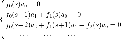
Thus the condition of satisfying the differential equation by (4) is the infinite system of
equations
 | | (6) |
In the first place, since a0≠0, the indicial equation
| f0(s) ≡ r0s2 + (p
0 − r0)s + q0 = 0 | | (7) |
must be satisfied. Because r0≠0, this quadratic equation determines for s two values, which in
special case may coincide.
The first of the equations (6) leaves a0 (≠0) arbitrary. The next linear equations in an
allow to solve successively the constants a1, a2, … provided that the first coefficients
f0(s+1), f0(s+2),… do not vanish; this is evidently the case when the roots of the
indicial equation don’t differ by an integer (e.g. when the roots are complex conjugates or
when s is the root having greater real part). In any case, one obtains at least for one of
the roots of the indicial equation the definite values of the coefficients an in the series
(4). It is not hard to show that then this series converges in a neighbourhood of the
origin.
For obtaining the complete solution of the differential equation (2) it suffices to have only one
solution y1(x) of the form (4), because another solution y2(x), linearly independent on y1(x), is
gotten via mere integrations; then it is possible in the cases s1−s2 ∈ ℤ that y2(x) has no
expansion of the form (4).
References
[1] Pentti Laasonen: Matemaattisia erikoisfunktioita. Handout No. 261. Teknillisen
Korkeakoulun Ylioppilaskunta; Otaniemi, Finland (1969).