|
|
|
|||||||
where
This equation describes the same mathematical structure that appears in first-order thermal models, simple electrical circuits, mixing problems, and many other relaxation processes.
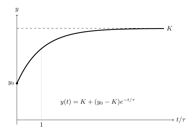
Figure 1. A generic first-order relaxation system. The state begins at y0 and approaches the steady value K with characteristic time scale τ.
1 What should the answer look like before we solve anything?At steady state, the derivative vanishes:
Equation (1) then gives
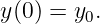
So the solution should approach K as time becomes large. At t = 0, the solution must satisfy
We therefore expect a transient that connects y0 to K.
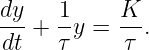
2 Direct time-domain solutionDivide Equation (1) by τ:
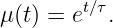
The integrating factor is
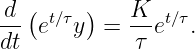
Multiply Equation (5) by this factor:
The left side is one derivative:
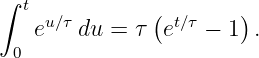
Integrate from 0 to t:
The integral is
Therefore
Rearrange:
Finally,
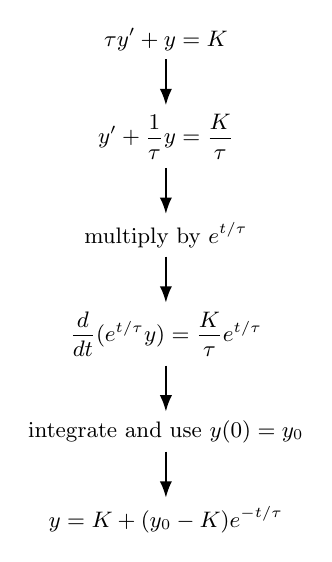
Figure 2. Direct time-domain route. Normalize the ODE, choose an integrating factor, combine the left side into one derivative, integrate, apply the initial value, and simplify.
3 Interpret the direct solutionEquation (13) separates naturally into
The steady part is
The transient is
At t = 0,
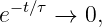
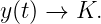
As t →∞,
so
The time constant controls how rapidly the transient decays. At
the transient has been reduced by the factor
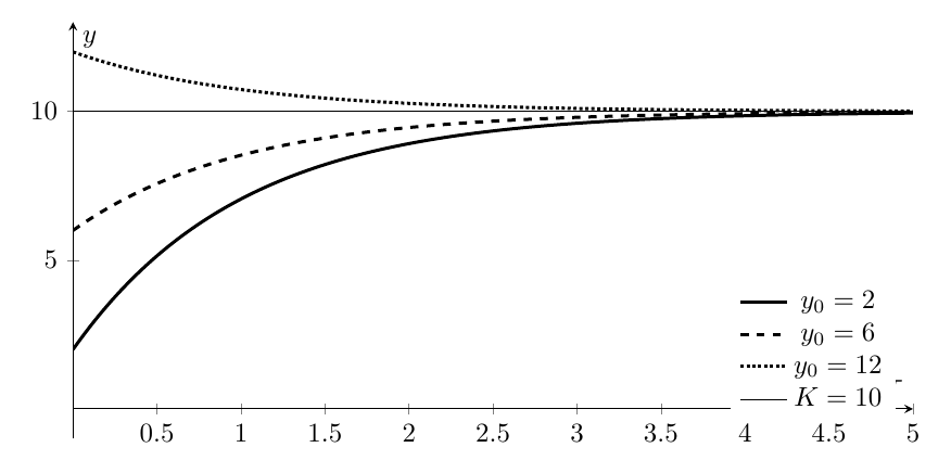
Figure 3. First-order relaxation for several initial values with the same K and τ. Every trajectory approaches the same steady value, while the exponential transient carries the memory of the initial condition.
4 Now solve the same problem using a Laplace-transform previewThe detailed transform rules will be derived later in the LT series. Here we use two results only to compare the structure of the calculation. Let
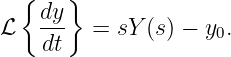
The derivative property is previewed as
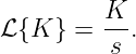
The transform of the constant forcing is
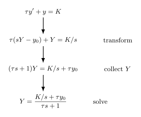
Apply the transform to
Using linearity,
Collect Y (s):
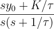
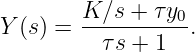
Solve algebraically:
The differential equation has disappeared. The unknown transform Y (s) is now found by ordinary algebra.
Figure 4. Transform-domain route. The derivative becomes sY − y0, the initial value appears immediately, and the ODE reduces to an algebraic equation for Y (s).
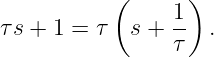
5 Rewrite the transform so the time-domain pieces are visibleStarting from Equation (28), use
Then
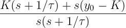
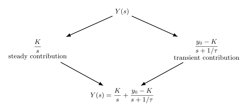
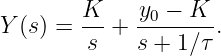
A particularly useful rearrangement is
To verify this, combine the right side:
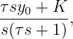
Multiplying numerator and denominator by τ gives
which matches Equation (28).
Figure 5. Algebraic decomposition of Y (s). The transform separates into a steady term K∕s and a transient term with denominator s + 1∕τ.
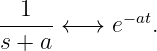
6 Return to the time domainThe two inverse-transform pairs used here are
and
Therefore Equation (31) gives
This is exactly the direct result in Equation (13).
7 Compare the two routesThe direct route required
The transform route required
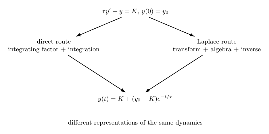
For this very simple problem, the direct method is not inferior. In fact, it is probably shorter. The advantage of the transform method becomes clearer when the forcing is delayed, piecewise, impulsive, or when several initial conditions and higher derivatives appear.
Figure 6. Two routes to the same solution. The direct method emphasizes integration in time; the Laplace route reorganizes the problem into algebra and then returns to time.
8 A numerical exampleLet
Then
At t = 0,
At one time constant,
At two time constants,
At three time constants,
The system approaches K = 10 exponentially.
9 What this example is meant to teachThis example should not yet be memorized as a collection of transform rules. Its purpose is to make three structural ideas concrete:
The remaining LT articles will derive the transform rules that were only previewed here.
10 Self-check questions
References
"First-Order Relaxation - Direct Solution and Laplace-Transform Preview" is owned by bloftin.
This object's parent. Cross-references: functions, domain, algebraic, differential equation, LT, representation, system This is version 1 of First-Order Relaxation - Direct Solution and Laplace-Transform Preview, born on 2026-10-31. Object id is 1544, canonical name is FirstOrderRelaxationDirectSolutionAndLaplaceTransformPreview. Accessed 3 times total. Classification:
|
|
|
|
Pending Errata and AddendaNone.
|
DiscussionNo messages.
|
Interact |




















 +