Calculus of Variations: Variations and the First Variation

CV01 established the setting of the classical variational problem. A functional acts on an admissible class of functions, and local optimality must be defined relative to a chosen neighborhood in function space. The next question is the analogue of ordinary differentiation:

If one perturbs an admissible function slightly, how does the scalar value of J change?

The central idea is to convert an infinite-dimensional problem into a one-parameter problem. Instead of trying to vary a function in all possible ways at once, one chooses a single admissible perturbation shape η(x) and studies the family

y (x) = y(x ) + 𝜖η(x). 𝜖

(1)

For fixed y and η, the functional becomes an ordinary scalar function of 𝜖,

Φ (𝜖) = J[y + 𝜖η ].

(2)

The derivative of Φ at 𝜖 = 0 is the first variation. It plays the role that f′(x_∗) plays in ordinary calculus. If y is a local extremum, the first variation must vanish for every admissible direction η.

This entry makes that construction precise, derives the standard first variation formula for first-order integral functionals, and works several examples in full detail. The next two entries will then use integration by parts and the Fundamental Lemma to pass from the vanishing of the first variation to the Euler–Lagrange equation.

1 Learning objectives

After this entry, the reader should be able to

define a variation and an admissible one-parameter family y_𝜖 = y + 𝜖η;
explain why endpoint conditions on y induce endpoint conditions on η;
define the scalar reduction Φ(𝜖) = J[y + 𝜖η];
define the first variation δJ[y; η] as a directional derivative;
derive the first variation formula for J[y] = ∫ _a^bF(x,y,y′) dx;
state clearly where differentiation under the integral sign is used;
prove that the first variation is linear in η;
compute first variations directly by expansion in 𝜖;
recognize that stationarity requires δJ[y; η] = 0 for every admissible η;
distinguish the first variation from the second variation; and
see how the first variation formula is poised for integration by parts and the Fundamental Lemma.

2 Variations as admissible perturbation directions

Let 𝒜 be an admissible class for a first-order problem. A variation is a comparison direction η(x) used to perturb a candidate function y(x).

The classical perturbed family is

y𝜖(x) = y(x ) + 𝜖η(x),

(3)

where 𝜖 ∈ ℝ is small.

The word “small” has two roles. First, it keeps y_𝜖 near y in whatever topology is relevant to the problem. Second, it allows one to use ordinary differentiation with respect to the scalar parameter 𝜖.

A variation must be chosen so that, for sufficiently small 𝜖, the perturbed curve remains admissible. Thus the admissibility conditions on y induce admissibility conditions on η.

2.1 Fixed endpoint problems

Suppose the admissible class is

{ } 𝒜 = y ∈ C1([a,b]) : y (a) = A, y(b) = B .

(4)

If y_𝜖 = y + 𝜖η is to satisfy the same endpoint conditions for all sufficiently small 𝜖, then

y𝜖(a) = A, y𝜖(b) = B.

(5)

Substituting the perturbed family gives

y(a) + 𝜖η(a) = A, y(b) + 𝜖η(b) = B.

(6)

Because y is already admissible, y(a) = A and y(b) = B, so one obtains

η (a ) = 0, η(b) = 0.

(7)

Thus, for fixed-endpoint problems, admissible variations vanish at the endpoints.

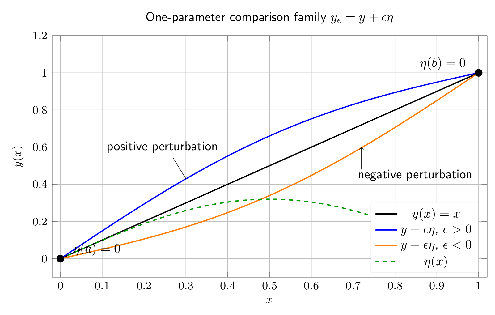
Figure. A typical one-parameter family y_𝜖 = y + 𝜖η for a fixed-endpoint problem. The comparison curves share the same endpoints because the variation η vanishes at x = a and x = b.

2.2 Other constraints

If the admissible class includes different constraints, the variation must respect them in the corresponding linearized sense.

For periodic constraints y(a) = y(b), one requires η(a) = η(b).
For an integral constraint such as ∫ _a^bG(x,y,y′) dx = C, not every η is immediately admissible; this issue leads to constrained variations and Lagrange multipliers in later entries.
For inequality or obstacle constraints, the admissible directions may be one-sided rather than arbitrary.

For the present entry, fixed-endpoint unconstrained problems are sufficient to show the core mechanism.

3 From an infinite-dimensional problem to an ordinary derivative

The first conceptual simplification in the calculus of variations is the map

y −→ {y + 𝜖η : 𝜖 ∈ ℝ } − → Φ(𝜖) = J[y + 𝜖η].

(8)

Once y and η are fixed, the functional no longer acts on an entire class of functions. It acts on a one-parameter subfamily. Along that subfamily the problem is ordinary calculus.

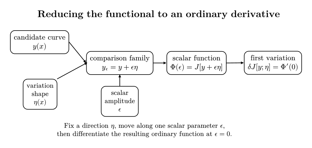
Figure. The standard reduction. A direction η and scalar amplitude 𝜖 produce a comparison family y + 𝜖η. The functional then becomes the ordinary scalar function Φ(𝜖) = J[y + 𝜖η]. Differentiating at 𝜖 = 0 yields the first variation.

3.1 Definition of the first variation

Let J be a functional and suppose the derivative exists. The first variation of J at y in the direction η is

d || δJ[y;η] = --J [y + 𝜖η ]|| . d𝜖 𝜖=0

(9)

Equivalently, if

Φ (𝜖) = J[y + 𝜖η ],

(10)

then

′ δJ[y;η] = Φ (0).

(11)

This is the classical Gâteaux or directional derivative viewpoint. One does not yet require the stronger uniform approximation property associated with the Fréchet derivative. For deriving the Euler–Lagrange equation, the directional viewpoint is the natural starting point.

3.2 Stationarity as an infinite-dimensional Fermat principle

In ordinary calculus, if x_∗ is an interior local extremum of a differentiable function f, then

f ′(x∗) = 0.

(12)

In several variables, if x_∗ is an interior local extremum of a smooth function f(x), then

∇f (x∗) = 0.

(13)

The analogous variational principle is:

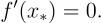
If y_∗ is a local extremum of J, then for every admissible variation η,

$δJ [y∗;η ] = 0.$ (14)

The crucial phrase is “for every admissible variation.” A single vanishing value of δJ[y; η] along one direction says very little. A local extremum must be stationary with respect to all admissible first-order perturbations.

4 First variation of a first-order integral functional

Consider the classical functional

∫ b ′ J[y] = F (x,y(x),y (x)) dx, a

(15)

where F is continuously differentiable in its arguments and y,η are sufficiently smooth for the expressions below to make sense.

Set

y𝜖 = y + 𝜖η, y′𝜖 = y ′ + 𝜖η′.

(16)

Then

∫ b ′ ′ Φ(𝜖) = J[y + 𝜖η] = a F (x,y + 𝜖η,y + 𝜖η )dx.

(17)

4.1 Main formula

proposition. Assume that F ∈ C¹ and that differentiation under the integral sign is justified for the perturbed family. Then the first variation is

|----------∫-------------------| | b ′ | |δJ[y;η] = (Fy η + Fy′ η )dx| ------------a-------------------

(18)

where F_y and F_y′ are evaluated along the unperturbed curve (x,y(x),y′(x)).

4.2 Proof

Differentiate Φ(𝜖) with respect to 𝜖:

∫ ′ d-- b ′ ′ Φ (𝜖) = d𝜖 F (x,y + 𝜖η,y + 𝜖η )dx. a

(19)

Assuming differentiation may pass under the integral sign,

∫ b Φ ′(𝜖) = -∂-F (x,y + 𝜖η,y′ + 𝜖η′)dx. a ∂ 𝜖

(20)

Now apply the chain rule to the integrand. Since x is independent of 𝜖,

∂ ′ ′ ′ ′ ′ ′ ′ --F (x,y + 𝜖η,y + 𝜖η ) = Fy(x, y + 𝜖η, y + 𝜖η )η + Fy′(x,y + 𝜖η,y + 𝜖η )η . ∂𝜖

(21)

Hence

∫ b Φ′(𝜖) = [F (x,y + 𝜖η,y′ + 𝜖η ′)η + F ′(x,y + 𝜖η,y ′ + 𝜖η′)η′]dx. a y y

(22)

Evaluating at 𝜖 = 0 gives

∫ ′ b ′ ′ ′ δJ[y;η] = Φ (0) = (Fy (x,y,y )η + Fy′(x, y,y)η )dx, a

(23)

which is the claimed formula.

4.3 Why the proof is important

The proof shows exactly where the machinery comes from. The first variation is not a mysterious formal symbol. It is an ordinary derivative with respect to 𝜖 after one restricts the functional to a one-parameter family.

The proof also isolates the analytic step that needs hypotheses: differentiation under the integral sign. In classical coursework one usually assumes enough smoothness for this to be valid. More advanced functional analysis develops sharper conditions, but the basic variational idea is already visible in the classical setting.

5 Linearity of the first variation

For fixed y, the map ηδJ[y; η] is linear.

Proposition. Let α,β ∈ ℝ and let η₁,η₂ be admissible variations. Then

δJ[y;α η1 + β η2] = α δJ [y; η1] + β δJ[y;η2].

(24)

Proof. Apply the first variation formula:

∫ b δJ[y;α η1 + β η2] = [Fy(αη1 + βη2) + Fy′(αη′1 + βη ′2)]dx. a

(25)

Distribute and use linearity of the integral:

∫ ∫ b ′ b ′ δJ[y;α η1 + β η2] = α (Fy η1 + Fy′η1)dx + β (Fyη2 + Fy ′η2)dx. a a

(26)

Therefore

δJ[y;α η1 + β η2] = α δJ [y; η1] + β δJ[y;η2].

(27)

This linearity is the reason one can think of δJ[y; ⋅] as an analogue of a differential or covector acting on perturbation directions.

6 Direct computation by 𝜖-expansion

Although the general formula is fundamental, students should be able to compute first variations directly from the definition. Expanding J[y + 𝜖η] in powers of 𝜖 is often the clearest way to see what is happening.

6.1 Example 1: the standard energy functional around the straight line

Consider

∫ 1 J[y] = y′(x)2dx, 0

(28)

with fixed endpoints

y (0 ) = 0, y(1) = 1.

(29)

Take the candidate

y(x) = x,

(30)

and the admissible variation

η(x) = sin(πx ),

(31)

which satisfies η(0) = η(1) = 0.

The perturbed family is

y𝜖(x) = x + 𝜖sin(πx ),

(32)

y ′𝜖(x) = 1 + 𝜖π cos(πx).

(33)

Substitute into J:

∫ 1 2 Φ (𝜖) = J[y𝜖] = (1 + 𝜖π cos(πx )) dx. 0

(34)

Expand the square:

∫ 1 ∫ 1 Φ (𝜖) = 1 + 2𝜖π cos(πx )dx + 𝜖2π2 cos2(πx )dx. 0 0

(35)

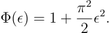
The middle integral vanishes and the last integral equals 1∕2, hence

π2 Φ (𝜖) = 1 + --𝜖2. 2

(36)

Therefore

δJ[y;η] = Φ′(0) = 0.

(37)

This shows that the straight line is stationary in the direction η(x) = sin(πx). In fact it is stationary for every admissible η, which will become completely transparent after integration by parts in CV04.

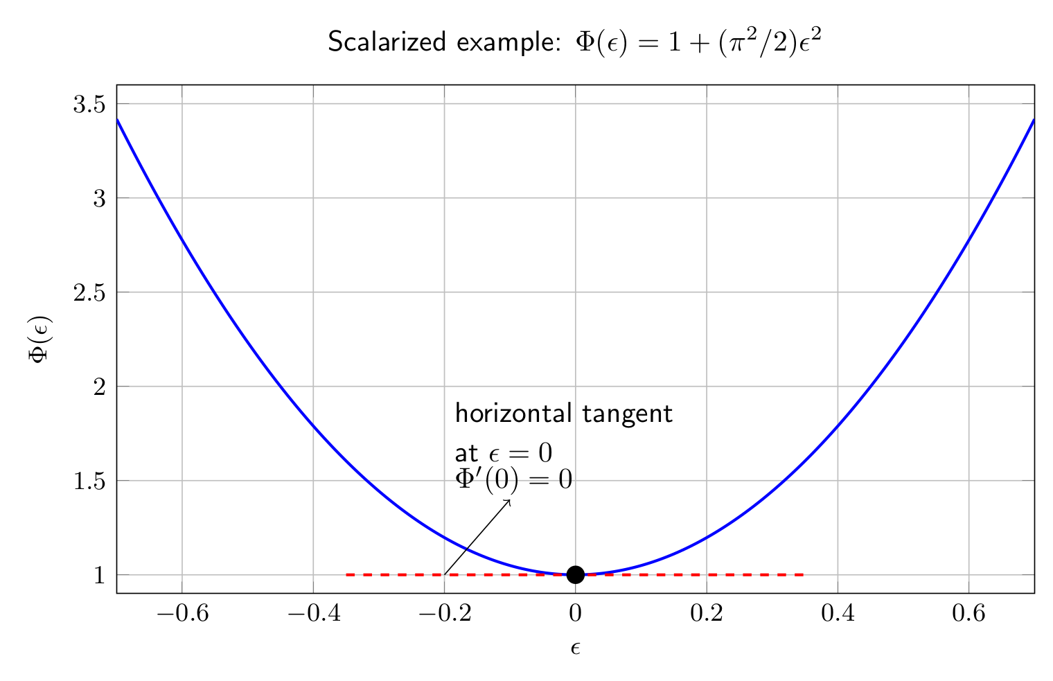
Figure. For the family y_𝜖 = x + 𝜖 sin(πx), the scalarized functional is Φ(𝜖) = 1 + (π²∕2)𝜖². The tangent at 𝜖 = 0 is horizontal, so the first variation vanishes.

6.2 Example 2: use the general formula

Now compute the same first variation from the formula. Here

F(x, y,y′) = y ′2.

(38)

Therefore

′ Fy = 0, Fy′ = 2y .

(39)

The first variation at a general admissible curve y is

∫ 1 δJ[y;η] = 2y ′η′dx. 0

(40)

For y(x) = x, one has y′ = 1, so

∫ 1 ′ 1 δJ[x;η] = 2 η (x )dx = 2 [η(x )]0 = 0. 0

(41)

Thus the straight line is stationary for every fixed-endpoint variation, as expected.

6.3 Example 3: a nonstationary admissible curve

Still with

∫ 1 J [y ] = y′2 dx, 0

(42)

consider the admissible curve

y(x) = x2,

(43)

which satisfies y(0) = 0 and y(1) = 1.

Choose the admissible variation

η(x) = x(1 − x).

(44)

Then

′ ′ y (x) = 2x, η (x) = 1 − 2x.

(45)

Using the formula,

∫ ∫ 1 ′ ′ 1 δJ[y;η] = 2 y η dx = 2 2x (1 − 2x)dx. 0 0

(46)

Compute the integral:

∫ 1 ( ) δJ[y;η] = 4 (x − 2x2)dx = 4 1-− 2- = − 2-. 0 2 3 3

(47)

Because the first variation is not zero, the curve y = x² is not stationary. So one does not need the full Euler–Lagrange equation merely to rule out a candidate. A single admissible direction with nonzero first variation is already enough.

6.4 Example 4: a functional containing both y and y′

Consider

∫ 1( ) J[y] = y2 + y′2 dx, 0

(48)

with fixed endpoints y(0) = y(1) = 0 and candidate y(x) = 0.

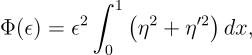
Let η be any admissible variation, so η(0) = η(1) = 0. Then

∫ ∫ 1( 2 2 2 ′2) 2 1( 2 ′2) J [𝜖η] = 𝜖η + 𝜖 η dx = 𝜖 η + η dx. 0 0

(49)

Hence

∫ 1 ( ) Φ(𝜖) = 𝜖2 η2 + η′2 dx, 0

(50)

δJ[0;η] = Φ′(0) = 0.

(51)

This example is useful because it shows that the first variation alone detects stationarity, not the full classification. Here the absence of a linear term already suggests that y = 0 should be minimizing, but one needs second-order information to establish that rigorously in general.

7 The bridge to Euler–Lagrange

The first variation formula still contains η′:

∫ b ′ δJ[y;η] = a (Fy η + Fy′η )dx.

(52)

The next step is to remove the derivative from the variation by integration by parts:

∫ ∫ b ′ b b-d- Fy′η dx = [Fy′η]a − dx (Fy′)η dx. a a

(53)

Substituting gives

∫ b( ) δJ[y;η] = [Fy ′η]ba + Fy − -d-Fy′ η dx. a dx

(54)

For fixed-endpoint variations, η(a) = η(b) = 0, so the boundary term drops out and one obtains

∫ b( d ) δJ [y;η ] = Fy − --Fy ′ η dx. a dx

(55)

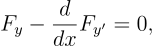
Now the structure is clear. If y is stationary, then this integral vanishes for every admissible variation η. The Fundamental Lemma will then imply

-d- Fy − dx Fy′ = 0,

(56)

which is the Euler–Lagrange equation.

This logical order matters:

|---------------------------------------------------------------------------------------------------| |variation family − → first variation −→ integration by parts −→ Fundamental Lemma −→ Euler–Lagrange | -----------------------------------------------------------------------------------------------------

(57)

CV03 is devoted to the Fundamental Lemma because that final implication is a nontrivial theorem, not a formal trick.

8 Common misconceptions

8.1 Misconception 1: the variation η is itself the new curve

No. The perturbed curve is y + 𝜖η. The function η provides the shape of the perturbation, while 𝜖 controls its size.

8.2 Misconception 2: if one example gives δJ = 0, the curve is stationary

No. Stationarity requires

δJ [y;η] = 0 for every admissible η.

(58)

A single direction is not enough.

8.3 Misconception 3: the first variation already proves a minimum

Not in general. Vanishing first variation is a necessary condition for an interior local extremum, but not a sufficient one. Classification belongs to second-variation theory.

8.4 Misconception 4: the first variation formula is obtained by formally “varying” symbols

The formula does have a compact formal notation, but its basis is ordinary calculus on the scalar function Φ(𝜖) = J[y + 𝜖η].

8.5 Misconception 5: differentiation under the integral sign is automatic

One needs hypotheses to justify it. In introductory classical treatments the required regularity is usually assumed from the start.

9 Compact definition table


Object	Meaning

η(x)	variation or perturbation direction

y_𝜖 = y + 𝜖η	one-parameter family of nearby curves

Φ(𝜖) = J[y + 𝜖η]	scalarized functional along one family

δJ[y; η]	first variation, equal to Φ′(0)

δ²J	second variation, based on Φ′′(0)

stationary function	one for which δJ[y; η] = 0 for all admissible η

10 What CV03 and CV04 add

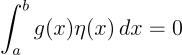
CV03 will prove the Fundamental Lemma of the Calculus of Variations. That lemma tells us that if

∫ b g(x)η(x)dx = 0 a

(59)

for every smooth test function η with compact support or vanishing endpoints, then g(x) = 0 identically.

CV04 will combine that lemma with the integration-by-parts form of the first variation to obtain the Euler–Lagrange equation in its standard classical form.

Thus CV02 provides the derivative computation, CV03 provides the theorem that converts an integral identity into a pointwise statement, and CV04 assembles those pieces into the central necessary condition of the subject.

11 Summary

The first variation is the directional derivative of a functional. Starting from a candidate y and an admissible variation η, one builds the family y + 𝜖η and defines

| -d- || δJ[y;η] = d𝜖J [y + 𝜖η ]| . 𝜖=0

(60)

For the classical first-order functional

∫ b J[y] = F (x,y,y′)dx, a

(61)

the first variation is

∫ b ′ δJ[y;η] = (Fy η + Fy′η )dx. a

(62)

This quantity is linear in the variation direction and must vanish for every admissible variation if y is a stationary function.

The first variation therefore plays the same conceptual role in the calculus of variations that the ordinary derivative plays in finite-dimensional calculus. Its integration-by-parts form is the gateway to the Fundamental Lemma and the Euler–Lagrange equation.

12 References and further reading

The following references are standard classical entry points into the subject. They are listed here for mathematical orientation; the present article remains self-contained.

I. M. Gelfand and S. V. Fomin, Calculus of Variations.
B. van Brunt, The Calculus of Variations.
C. Fox, An Introduction to the Calculus of Variations.
L. C. Evans, Partial Differential Equations, for the modern weak and functional-analytic viewpoint.
H. Goldstein, C. Poole, and J. Safko, Classical Mechanics, for the action principle connection.

"Calculus of Variations: Variations and the First Variation" is owned by bloftin.
(view preamble)