Orbital Plane to Inertial Coordinates: The PQW-to-ECI Transformation

1 Why another coordinate frame is needed

In a two-body orbit, the simplest coordinates are attached directly to the orbital geometry. GPSORB04 derived the conic orbit

p r = ----------, p = a(1 − e2), 1 + ecos ν

(1)

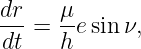
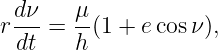
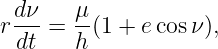
and GPSORB06 showed how the true anomaly ν evolves through the chain

t − → M −→ E − → ν.

(2)

Once r and ν are known, the satellite position in its own orbital plane is almost trivial.

The problem is that an orbital-plane coordinate system is different for every orbit. A GPS receiver, a tracking station, or a multi-satellite orbit-determination program needs all satellite states represented in a common frame. The natural intermediate frame is an Earth-centered inertial frame, abbreviated ECI.

The essential transformation is therefore

|----------------------------------------------------------------| |orbital- plane coordinates − → inertial Cartesian coordinates. | -----------------------------------------------------------------

(3)

The three classical orientation elements Ω, i, and ω are precisely the three angles required to perform this transformation.

2 The two frames

2.1 The inertial frame

Let the Earth-centered inertial frame have orthonormal basis vectors

^I, ^J, ^K.

(4)

The Z axis is aligned with the chosen inertial reference pole and the X axis defines the inertial reference direction. The XY plane is therefore the inertial reference plane.

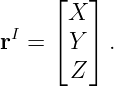
A Cartesian position vector resolved in this frame is written

⌊ ⌋ X rI = ⌈ Y ⌉ . Z

(5)

2.2 The perifocal frame

The orbital-plane frame is usually called the perifocal or PQW frame. Its basis vectors are

^ ^ ^ P, Q, W.

(6)

They are defined physically:

P points from the occupied focus toward periapsis.
Q lies in the orbital plane, 90^∘ ahead of P in the direction of motion.
W = h is normal to the orbital plane in the direction of the specific angular-momentum vector.

Thus

^P × ^Q = ^W.

(7)

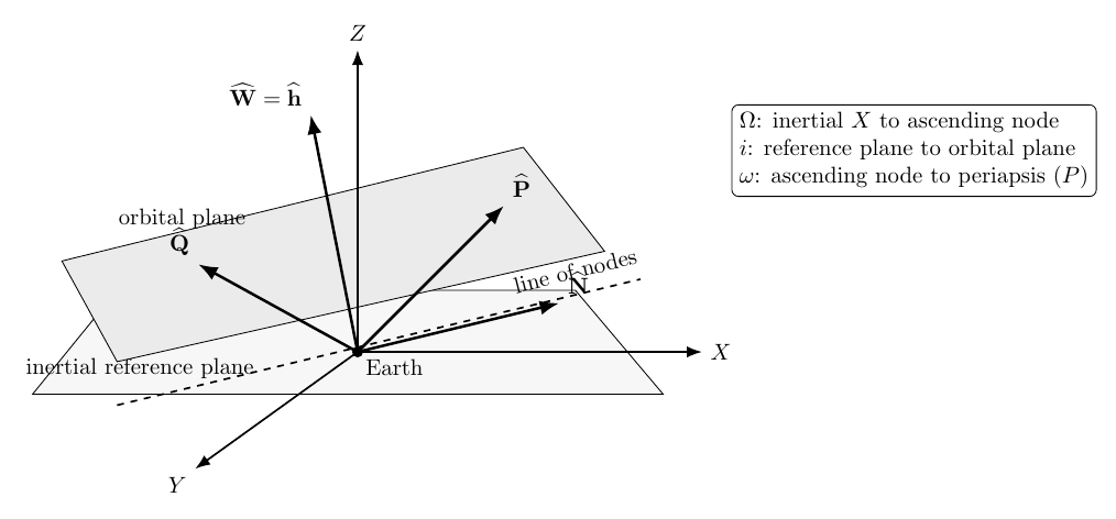
Figure 1. The inertial and perifocal frames are related by the node angle, inclination, and periapsis angle.

The three orientation elements have distinct geometric roles. The right ascension of the ascending node Ω fixes the direction of the line of nodes in the inertial reference plane. The inclination i tilts the orbital plane away from the reference plane. The argument of periapsis ω rotates within the orbital plane from the ascending node to the periapsis direction.

3 Position and velocity in the perifocal frame

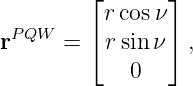
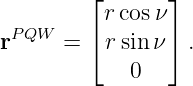
Because the P axis points toward periapsis, true anomaly ν is measured directly from the P axis. Therefore

⌊ ⌋ r cosν rP QW = ⌈r sin ν⌉ . 0

(8)

The third component is zero because the satellite lies in the orbital plane.

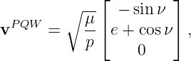
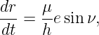
Using the radial and transverse velocity components derived in GPSORB04,

dr μ ---= -e sin ν, dt h

(9)

and

d-ν μ- r dt = h (1 + ecosν ),

(10)

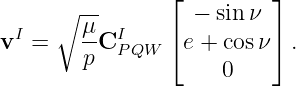
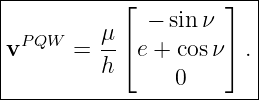
one obtains the standard perifocal velocity vector

|-----------⌊---------⌋--| | − sin ν | |vP QW = μ-⌈e + cos ν⌉ .| | h 0 | -------------------------|

(11)

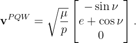
Since p = h²∕μ,

∘ -- μ-= μ-, h p

(12)

so Eq. (11) is often written

⌊ ⌋ ∘ μ- − sin ν vPQW = --⌈ e + cos ν⌉ . p 0

(13)

At this point all orbital dynamics are contained in r, ν, and the scalar orbital parameters. The remaining problem is purely geometric: rotate these vectors into the inertial basis.

4 Transformation convention

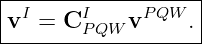
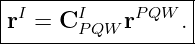
Rotation formulas are a frequent source of sign and transpose errors, so the mapping used here is defined explicitly:

|------------------| |rI = CIPQW rPQW .| -------------------

(14)

The superscript I means that the result is resolved in inertial coordinates; the subscript PQW identifies the source components.

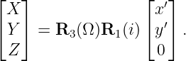
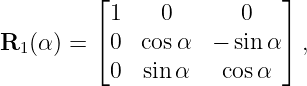
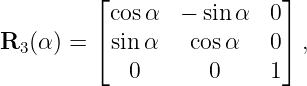
With the standard right-handed active rotation matrices

⌊ ⌋ 1 0 0 R1 (α) = ⌈0 cos α − sinα ⌉ , 0 sin α cosα

(15)

and

⌊cos α − sinα 0⌋ ⌈ ⌉ R3 (α) = sin α cosα 0 , 0 0 1

(16)

the required mapping is

|----------------------------| |CIPQW = R3 (Ω)R1 (i)R3(ω ).| -----------------------------

(17)

Figure 2. Matrix factors for the perifocal-to-inertial mapping used in this article.

For column vectors, the rightmost matrix acts first. In attitude literature one may encounter passive coordinate transformations using the opposite direction. For the reverse mapping in the present convention,

rP QW = (CI )TrI. PQW

(18)

Because a proper rotation matrix is orthogonal, transpose and inverse are identical.

5 A geometric derivation from the line of nodes

Before multiplying matrices, it is useful to build the perifocal basis directly from the orbital geometry. This makes the meaning of every column in the transformation matrix explicit.

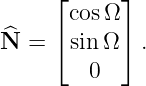
The unit vector along the ascending-node direction is

⌊ ⌋ cos Ω ^N = ⌈sinΩ ⌉ . 0

(19)

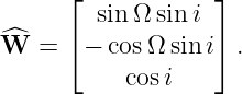
The unit orbit normal follows from the familiar inclination and node geometry:

⌊ sin Ω sin i ⌋ ^ ⌈ ⌉ W = − cos Ω sin i . cosi

(20)

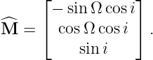
A second unit vector in the orbital plane, perpendicular to the node direction, is

^M = ^W × ^N.

(21)

Evaluating the cross product gives

⌊ ⌋ − sinΩ cos i ^M = ⌈ cosΩ cos i ⌉. sin i

(22)

The pair N,M therefore forms an orthonormal basis in the orbital plane, with N pointing toward the ascending node.

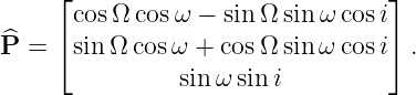
Periapsis is rotated by ω from the ascending-node direction, so

|-----------------------| ^P = cosω N^ + sin ω ^M. | -------------------------

(23)

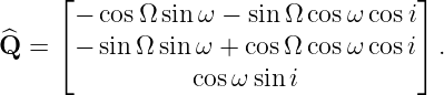
The Q direction is 90^∘ farther in the positive orbital direction:

|--------------------------| |^ ^ ^ | -Q--=-−-sinω-N--+-cosω-M.--

(24)

Substituting Eqs. (19) and (22) into Eq. (23),

⌊ ⌋ cosΩ cos ω − sin Ω sinω cosi ^P = ⌈ sin Ω cosω + cosΩ sin ω cosi⌉ . sinω sini

(25)

Similarly,

⌊ − cosΩ sin ω − sin Ω cosω cos i⌋ ^ Q = ⌈ − sinΩ sinω + cosΩ cosω cos i⌉ . cosω sini

(26)

The third basis vector is Eq. (20).

The transformation matrix can now be read off directly:

|------------------------| | [ | | | ] | |CIPQW = ^P Q^ ^W .| | | | | | -------------------------

(27)

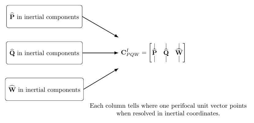
Figure 3. The transformation matrix columns are the perifocal basis vectors resolved in inertial coordinates.

This column interpretation is one of the most useful ways to understand a direction cosine matrix. Multiplying by the coordinate vector [r_P,r_Q,r_W]^T simply forms

rI = rPP^ + rQQ^ + rW ^W.

(28)

6 Matrix derivation

Now derive the same result algebraically. First multiply the two rightmost matrices:

⌊ cos ω − sin ω 0 ⌋ ⌈ ⌉ R1 (i)R3(ω ) = cosi sin ω cos icosω − sin i . sini sin ω sini cosω cos i

(29)

Premultiplying by R₃(Ω) gives

⌊ ⌋ cΩcω − sΩsωci − cΩsω − sΩcωci sΩsi CI = ⌈ sΩcω + cΩsωci − sΩsω + cΩcωci − cΩsi⌉ , PQW s s c s c ω i ω i i

(30)

where, for compactness,

cΩ = cosΩ, sΩ = sin Ω, ci = cosi, si = sini,

(31)

and similarly for c_ω and s_ω.

Equation (30) is identical to the matrix obtained from the geometric basis-vector derivation. This agreement is an important check: the matrix is not an arbitrary collection of trigonometric terms. Every column has a direct geometric meaning.

7 Transforming the position vector

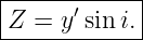
Substitute Eq. (8) into Eq. (14). Because the third perifocal coordinate is zero,

rI = r cosν ^P + r sin νQ^.

(32)

Expanding the first component gives

X = rcos ν(cosΩ cos ω − sin Ω sinω cosi) + rsinν (− cosΩ sin ω − sinΩ cos ω cosi).

(33)

Group the cos Ω and sin Ω cos i terms:

X = r cosΩ (cosω cosν − sinω sinν ) − rsin Ω cosi(sin ω cosν + cosω sinν ).

(34)

Using the angle-addition identities,

cos(ω + ν) = cosω cos ν − sin ω sin ν,

(35)

and

sin (ω + ν) = sin ω cosν + cos ωsin ν.

(36)

Define the argument of latitude

|----------| u-=--ω-+-ν.-

(37)

Then

|------------------------------------| |X = r(cosΩ cos u − sin Ω sin u cosi).| -------------------------------------

(38)

The same process yields

|------------------------------------| |Y = r(sin Ω cosu + cos Ω sin u cosi),| -------------------------------------

(39)

and

|----------------| |Z = rsinu sin i.| -----------------

(40)

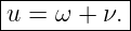
These three equations are worth understanding physically. The combination ω + ν appears because once the orbit has been rotated into its plane, the instantaneous satellite direction is measured from the ascending node by the total in-plane angle u.

8 A shorter two-rotation form using argument of latitude

Once u = ω + ν is known, it is not necessary to carry the periapsis rotation separately. Define in-plane coordinates measured from the ascending node:

′ ′ x = rcosu, y = rsin u.

(41)

Then

⌊ ⌋ ⌊ ⌋ X x′ ⌈Y ⌉ = R (Ω )R (i) ⌈y′⌉ . 3 1 Z 0

(42)

Expanding Eq. (42),

|----------------------------| -X--=-x′cos-Ω-−-y′cos-isin-Ω,-|

(43)

|---------------------------| Y = x′sinΩ + y′cosicos Ω, | -----------------------------

(44)

and

|------′-----| -Z-=--y-sin-i.|

(45)

These equations will later look very familiar when the GPS broadcast ephemeris is developed.

9 Transforming the velocity vector

The simplest velocity transformation uses the same constant rotation matrix:

|------------------| |vI = CIPQW vP QW .| --------------------

(46)

Substituting Eq. (11),

⌊ ⌋ ∘ μ- − sinν vI = --CIPQW ⌈ e + cosν⌉ . p 0

(47)

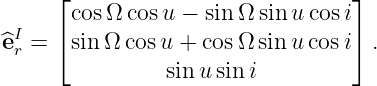
There is also a physically transparent radial-transverse form. The inertial radial unit vector is obtained by dividing Eqs. (38)–(40) by r:

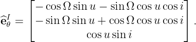
⌊cos Ω cosu − sinΩ sinu cosi⌋ I ⌈ ⌉ ^er = sinΩ cos u + cosΩ sinu cosi . sinu sini

(48)

The transverse unit vector is obtained by differentiating with respect to u:

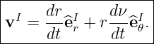
⌊ ⌋ − cos Ω sin u − sin Ω cosu cosi ^eI𝜃 = ⌈− sinΩ sin u + cosΩ cosu cosi⌉ . cos usini

(49)

Therefore

--------------------- | dr dν | |vI = ---^eIr + r---^eI𝜃.| -------dt------dt----|

(50)

For the unperturbed two-body problem, Ω, i, and ω are constant, so du∕dt = dν∕dt.

Using the two-body expressions

dr-= μe sin ν, dt h

(51)

and

d ν μ r--- = --(1 + ecosν ), dt h

(52)

Eq. (50) becomes completely determined by the orbital elements and current true anomaly.

10 Why the transpose gives the inverse transformation

The columns of C_PQW^I are orthonormal basis vectors, so

(CIP QW )TCIPQW = I.

(53)

Hence

(CI )−1 = (CI )T. PQW PQW

(54)

The determinant is

I det(C PQW ) = +1,

(55)

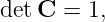
so this is a proper rotation, not a reflection.

These properties give valuable software tests. If a computed matrix significantly violates

T C C = I

(56)

detC = 1,

(57)

there is almost certainly a sign, angle-unit, or matrix-order error.

11 Sanity checks and limiting cases

Several special cases help verify the equations.

11.1 Zero node angle

If Ω = 0, the ascending node lies along the inertial X axis. Equations (38)–(40) reduce to

X = rcos u,

(58)

Y = rsin u cosi,

(59)

and

Z = rsinu sin i.

(60)

This is exactly the geometry of tilting the orbital plane about the X axis.

11.2 Zero inclination

If i = 0, then

Z = 0,

(61)

and the motion remains in the inertial reference plane. The horizontal coordinates become

X = rcos(Ω + u),

(62)

Y = rsin(Ω + u ).

(63)

Because an equatorial orbit has no unique ascending node, Ω and ω separately become singular, but their sum remains physically meaningful. This is the same singularity discussed in GPSORB05.

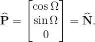
11.3 Zero argument of periapsis

If ω = 0, then P lies along the ascending-node direction. The P column of Eq. (30) reduces to

⌊ ⌋ cosΩ P^ = ⌈ sin Ω ⌉ = N^. 0

(64)

Again the geometry agrees with the element definition.

12 Worked GPS-like numerical example

Use the element set

a = 26560 km, e = 0.01,

(65)

i = 55∘, Ω = 40∘, ω = 30 ∘, ν = 70∘,

(66)

with

μ = 398600.4418 km3 ∕s2.

(67)

First compute

p = a(1 − e2) = 26557.344 km.

(68)

The orbital radius is

p r = ----------≈ 26466.8221 km. 1 + e cosν

(69)

Therefore

⌊ ⌋ 9052.1863 rPQW ≈ ⌈24870.6775 ⌉ km. 0

(70)

The specific angular momentum is

√ --- h = μp ≈ 102887.1666 km2 ∕s,

(71)

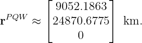
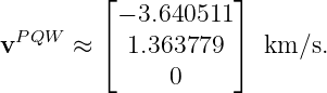
and the perifocal velocity is

⌊ ⌋ − 3.640511 vP QW ≈ ⌈ 1.363779 ⌉ km ∕s. 0

(72)

The transformation matrix evaluates to

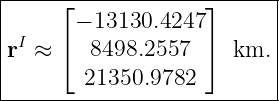
⌊ ⌋ 0.479070 − 0.702315 0.526541 CIP QW ≈ ⌈0.776363 0.059125 − 0.627507 ⌉ . 0.409576 0.709406 0.573576

(73)

Multiplying Eq. (73) by Eq. (70),

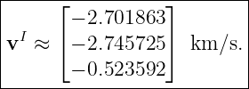
|-----⌊-------------⌋------| | − 13130.4247 | |rI ≈ ⌈ 8498.2557 ⌉ km. | | 21350.9782 | ---------------------------|

(74)

Similarly,

|-----⌊-----------⌋--------| | − 2.701863 | |vI ≈ ⌈ − 2.745725 ⌉ km ∕s.| | − 0.523592 | ---------------------------|

(75)

These are the same state vectors used in the worked inverse conversion of GPSORB05. Thus the forward and inverse mappings close the loop:

(r,v) ← → (a, e,i,Ω, ω, ν).

(76)

13 Connection to the GPS broadcast position equations

The GPS broadcast user algorithm eventually forms a corrected argument of latitude u_k, corrected radius r_k, corrected inclination i_k, and corrected node longitude Ω_k. It then defines orbital-plane coordinates

′ xk = rk cos uk,

(77)

y′k = rk sinuk.

(78)

The final coordinate equations have the same geometric structure as Eqs. (43)–(45):

xk = x ′k cosΩk − y′k cos ik sin Ωk,

(79)

yk = x ′k sin Ωk + y ′k cosik cos Ωk,

(80)

and

zk = y′k sin ik.

(81)

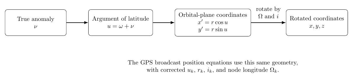
Figure 4. The argument-of-latitude form leads directly to the structure used in the GPS broadcast position equations.

There is, however, an important frame distinction. The derivation in this article has produced an inertial position when Ω is interpreted as an inertial node angle. The GPS broadcast algorithm is designed to deliver the satellite position in the WGS 84 Earth-centered Earth-fixed frame, so its node longitude contains Earth-rotation terms. That rotating-frame step is not hidden inside the present PQW-to-ECI derivation; it is a separate physical transformation and will be treated explicitly in the next stage of the series.

14 What has been accomplished

Starting with the natural orbital-plane state

⌊r cosν⌋ P QW ⌈ ⌉ r = r sin ν , 0

(82)

and

⌊ ⌋ ∘ μ- − sin ν vPQW = --⌈ e + cos ν⌉ , p 0

(83)

we derived the orientation matrix

I C PQW = R3 (Ω)R1 (i)R3(ω ),

(84)

its explicit components, and the equivalent basis-vector interpretation. The position formulas reduce naturally when the argument of latitude

u = ω + ν

(85)

is introduced, giving

X = r(cosΩ cos u − sin Ω sin u cosi),

(86)

Y = r(sin Ω cosu + cos Ω sin u cosi),

(87)

and

Z = rsinu sin i.

(88)

These equations provide the geometric bridge from Keplerian orbital elements to a common three-dimensional Cartesian frame. They also explain, rather than merely reproduce, the structure of the coordinate equations later used by the GPS broadcast ephemeris.

References

[1] E. D. Kaplan and C. J. Hegarty, eds., Understanding GPS/GNSS: Principles and Applications, 3rd ed., Artech House, 2017.

[2] D. A. Vallado, Fundamentals of Astrodynamics and Applications, 4th ed., Microcosm Press, 2013.

[3] H. D. Curtis, Orbital Mechanics for Engineering Students, 4th ed., Elsevier, 2020.

[4] R. R. Bate, D. D. Mueller, and J. E. White, Fundamentals of Astrodynamics, Dover Publications, 1971.

[5] U.S. Space Force, IS-GPS-200N: Navstar GPS Space Segment/Navigation User Interfaces, 1 August 2022, especially Table 20-IV.

"Orbital Plane to Inertial Coordinates: The PQW-to-ECI Transformation" is owned by bloftin.
(view preamble)