Electromagnetic Waves, Antennas, and RF: RF Interference and Jamming - Exercises

(Example)

Electromagnetic Waves, Antennas, and RF: RF Interference and Jamming - Exercises and Complete Worked Solutions

This companion to EM27 develops calculation skill with receiver-side interference metrics. The problems move from basic Power ratios to spectral overlap, equivalent noise bandwidth, receiver degradation, antenna discrimination, equivalent interference temperature, and a final GNSS-style allowable-interference calculation. The emphasis is defensive receiver analysis: all powers are referred to a common receiver plane and the limits of the additive-power model are stated explicitly [1, 2, 4, 5].

The principal relations are

( ) J- = J − S , S dB dBW dBW

(1)

( ) -J- N0 = JdBW − N0,dBW ∕Hz, dB−Hz

(2)

J J∕N0 ---= -----, N Bn

(3)

C C∕N -------= --------, N + J 1 + J∕N

(4)

and

( ) D = 10 log 1 + -J- . dB 10 N

(5)

For flat noise-like interference,

---C---- --C-∕N0--- N + J = 1 + J ∕N . 0 0 0 0

(6)

Use

k = 1.380649 × 10− 23J/K.

(7)

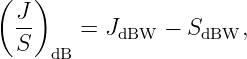
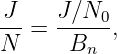
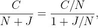
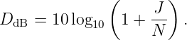
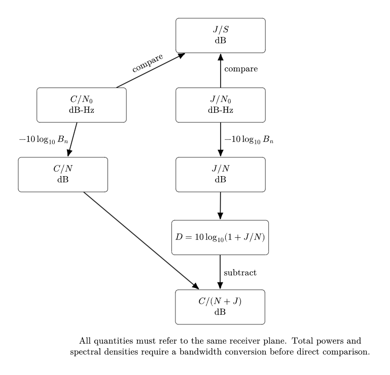
Figure 1. The main conversions used throughout the exercises. Total powers, spectral densities, and finite-bandwidth powers must not be mixed without the appropriate bandwidth conversion.

Part I: Exercises

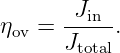
Exercise 1: interference-to-signal ratio

At a common receiver reference plane,

S = − 128 dBm, J = − 136 dBm.

(8)

Find J∕S in dB and linear form.

Exercise 2: J∕N₀ from system temperature

A receiver has

Tsys = 320 K

(9)

and admits an interference power

J = − 148 dBW.

(10)

Find N₀ in dBW/Hz and J∕N₀ in dB-Hz.

Exercise 3: convert C∕N₀ and J∕N₀ to J∕S

At the same reference plane,

C ∕N0 = 47 dB-Hz, J ∕N0 = 39 dB -Hz.

(11)

Assuming S = C, find J∕S.

Exercise 4: bandwidth conversion from J∕N₀ to J∕N

A receiver has

J ∕N = 53 dB -Hz, B = 200kHz. 0 n

(12)

Find J∕N in dB and linear form.

Exercise 5: additive interference degradation

A noise-only receiver has

C∕N = 12 dB.

(13)

An additive in-band interferer produces

J∕N = − 3dB.

(14)

Find the degradation D_dB and the resulting C∕(N + J).

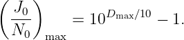
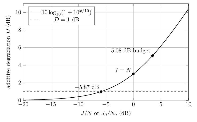
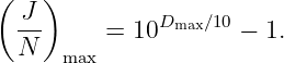
Exercise 6: invert a degradation requirement

Define an interference degradation budget D_max as the largest permitted additive degradation. For

Dmax = 1.00 dB,

(15)

find the largest allowable J∕N in linear form and in dB.

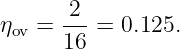
Exercise 7: broadband spectral overlap

A noise-like interferer has total received power

Jtotal = − 92dBm

(16)

uniformly distributed over 16 MHz. An ideal rectangular receiver admits 2 MHz entirely inside that band. Assume T = 290 K. Find:

admitted interference power J_in;
thermal-noise power N;
J∕N;
additive degradation D_dB.

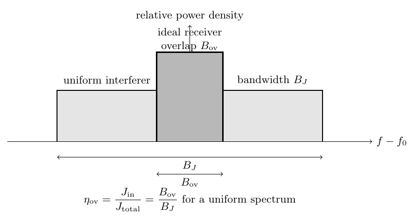
Figure 2. For a uniform broadband interferer and an ideal rectangular receiver, the admitted fraction equals the overlap bandwidth divided by the interference bandwidth.

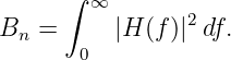
Exercise 8: equivalent noise bandwidth of a first-order low-pass filter

A one-sided normalized receiver power response is

|H (f)|2 = ----1------, f ≥ 0, 1 + (f ∕fc)2

(17)

with

fc = 100 kHz.

(18)

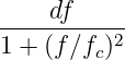
Find the one-sided equivalent noise bandwidth

∫ ∞ Bn = |H (f)|2df. 0

(19)

If a flat interference density is

J0 = − 175dBm/Hz,

(20)

find the admitted interference power and, at 290 K, the density-domain degradation.

Exercise 9: noise-like interference density

A receiver has

C ∕N0 = 46.5 dB -Hz

(21)

and a flat noise-like interference density satisfying

J0∕N0 = − 8 dB.

(22)

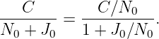
Find the degradation and the effective C∕(N₀ + J₀).

Exercise 10: equivalent interference temperature

A receiver has

Tsys = 350 K.

(23)

It admits

J = 2.0 × 10−15W

(24)

over

Bn = 2.0MHz.

(25)

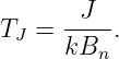
Find the equivalent interference temperature T_J, the effective temperature T_eff, and the corresponding degradation.

Exercise 11: two independent RF links

A desired transmitter and an interfering transmitter terminate at the same receiver. Their link terms are

EIRP_S	= 20 dBW,	L_S,path	= 140 dB,	L_S,other	= 2 dB,	G_r(Ω_S)	= 6 dBi,	(26)
EIRP_J	= 10 dBW,	L_J,path	= 132 dB,	L_J,other	= 1 dB,	G_r(Ω_J)	= −4 dBi.	(27)

Find S, J, and J∕S in dB.

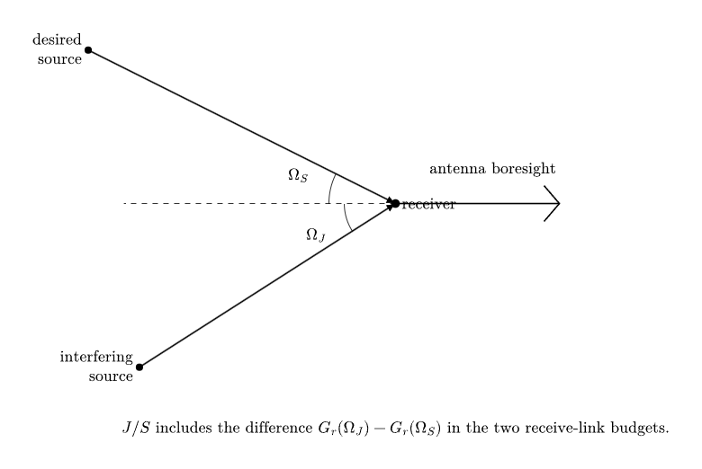
Exercise 12: receive-antenna interference discrimination

Before spatial discrimination, an interfering signal has

J∕S = − 3dB.

(28)

A directional receive antenna reduces the gain toward the interferer by 18 dB relative to the desired direction, with all other terms unchanged. Find the new J∕S. State how J∕N₀ changes if the receiver noise density at the chosen reference plane is unchanged.

Figure 3. Desired and interfering signals are separate links. Receive-antenna discrimination can change the interference power without changing the desired-signal path.

Exercise 13: combine C∕N₀, J∕N₀, and finite bandwidth

Let

C ∕N0 = 60 dB -Hz, J∕N0 = 55dB -Hz, Bn = 100 kHz.

(29)

Find C∕N, J∕N, the degradation, and C∕(N + J).

Exercise 14: same total interference power, different overlap

Two broadband interferers each arrive with total power

J = − 90dBm total

(30)

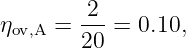
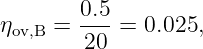
uniformly spread over 20 MHz. For interferer A, a 2 MHz receiver lies fully inside the interference band. For interferer B, only 0.5 MHz of the receiver passband overlaps the interference band. Find the admitted interference powers and their difference in dB.

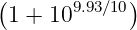
Exercise 15: GNSS-style density-domain degradation

An illustrative receiver has

C ∕N0 = 47.08 dB -Hz, J0∕N0 = − 6.0 dB.

(31)

For

Bn = 2.0MHz,

(32)

find the density-domain degradation, the effective C∕(N₀ + J₀), and the corresponding finite-bandwidth C∕(N + J).

Exercise 16: allowable noise-like interference from a receiver requirement

The same illustrative receiver has nominal

C∕N0 = 47.08dB -Hz

(33)

and must maintain

C ∕(N0 + J0) ≥ 42.00 dB-Hz.

(34)

Assuming additive uncorrelated noise-like interference, determine the maximum allowable J₀∕N₀ in linear form and in dB.

Figure 4. Additive degradation as a function of J∕N or, for flat noise-like interference, J₀∕N₀. The inverse relation converts a degradation budget into an allowable interference ratio.

Part II: Complete Worked Solutions

Solution 1: interference-to-signal ratio

Because both powers are expressed in the same logarithmic units at the same reference plane,

(J∕S)_dB	= J_dBm − S_dBm	(35)
	= −136 − (−128)	(36)
	= −8.00 dB.	(37)

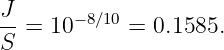
The linear ratio is

J-= 10−8∕10 = 0.1585. S

(38)

Thus the interference power is about 15.8% of the desired-signal power.

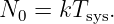
Solution 2: J∕N₀ from system temperature

The thermal-noise density is

N0 = kTsys.

(39)

In dBW/Hz,

N_0,dBW∕Hz	= 10 log ₁₀	(40)
	= −203.55 dBW/Hz.	(41)

Therefore

(J∕N₀)_dB−Hz	= −148 − (−203.55)	(42)
	= 55.55 dB-Hz.	(43)

Solution 3: convert C∕N₀ and J∕N₀ to J∕S

With S = C,

( ) ( ) ( ) J- -J- C-- S = N0 − N0 . dB dB−Hz dB− Hz

(44)

Hence

J ∕S = 39 − 47 = − 8.00 dB.

(45)

The dB-Hz units cancel because both ratios use the same N₀.

Solution 4: bandwidth conversion from J∕N₀ to J∕N

The bandwidth term is

10 log ₁₀B_n	= 10 log ₁₀(2.00 × 10⁵)	(46)
	= 53.0103 dB-Hz.	(47)

Therefore

(J∕N)_dB	= 53.00 − 53.0103	(48)
	= −0.0103 dB.	(49)

In linear form,

J∕N = 10− 0.0103∕10 = 0.9976.

(50)

The interference and thermal-noise powers are therefore almost equal.

Solution 5: additive interference degradation

First convert the interference ratio:

J∕N = 10−3∕10 = 0.5012.

(51)

The degradation is

D_dB	= 10 log ₁₀(1 + 0.5012)	(52)
	= 1.764 dB.	(53)

Therefore

C∕(N + J)_dB	= (C∕N)_dB − D_dB	(54)
	= 12.00 − 1.764	(55)
	= 10.236 dB.	(56)

Solution 6: invert a degradation requirement

Starting from

Dmax = 10log10(1 + J∕N ),

(57)

exponentiate both sides:

Dmax∕10 10 = 1 + J∕N.

(58)

Hence the largest allowable ratio is

( ) J-- Dmax∕10 N = 10 − 1. max

(59)

For D_max = 1.00 dB,

0.1 (J ∕N )max = 10 − 1 = 0.2589.

(60)

In decibels,

(J ∕N )max,dB = 10 log10(0.2589) = − 5.87dB.

(61)

Solution 7: broadband spectral overlap

For a uniform spectrum, define the spectral-overlap fraction

Jin ηov = J----. total

(62)

With complete containment of the receiver band,

-2- ηov = 16 = 0.125.

(63)

Thus

J_in,dBm	= −92 + 10 log ₁₀(0.125)	(64)
	= −101.03 dBm.	(65)

At 290 K,

N0,dBm∕Hz ≈ − 173.98dBm/Hz.

(66)

Therefore

N_dBm	= −173.98 + 10 log ₁₀(2.0 × 10⁶)	(67)
	= −110.96 dBm.	(68)

The ratio is

(J ∕N )dB = − 101.03 − (− 110.96) = 9.93dB.

(69)

The degradation is

D_dB	= 10 log ₁₀	(70)
	= 10.35 dB.	(71)

Solution 8: equivalent noise bandwidth of a first-order low-pass filter

The one-sided equivalent noise bandwidth is

B_n

= ∫ ₀^∞

(72)

Let u = f∕f_c, so df = f_c du. Then

B_n	= f_c ∫ ₀^∞	(73)
	= f_c₀^∞	(74)
	= f_c.	(75)

For f_c = 100 kHz,

Bn = 157.08 kHz.

(76)

The admitted flat-spectrum interference is

J_in,dBm	= J_0,dBm∕Hz + 10 log ₁₀B_n	(77)
	= −175 + 10 log ₁₀(1.5708 × 10⁵)	(78)
	= −123.04 dBm.	(79)

At 290 K,

N0 ≈ − 173.98 dBm/Hz,

(80)

(J0∕N0 )dB = − 175 − (− 173.98 ) = − 1.02 dB.

(81)

The density-domain degradation is therefore

( ) DdB = 10 log10 1 + 10−1.02∕10 = 2.53dB.

(82)

Solution 9: noise-like interference density

Convert the density ratio to linear form:

J ∕N = 10−8∕10 = 0.1585. 0 0

(83)

Then

D_dB	= 10 log ₁₀(1 + 0.1585)	(84)
	= 0.639 dB.	(85)

The effective density ratio is

C∕(N₀ + J₀)_dB−Hz	= 46.5 − 0.639	(86)
	= 45.86 dB-Hz.	(87)

Solution 10: equivalent interference temperature

By definition,

J TJ = ----. kBn

(88)

Thus

T_J	=	(89)
	= 72.43 K.	(90)

The effective temperature is

Teff = 350 + 72.43 = 422.43 K.

(91)

The degradation is

D_dB	= 10 log ₁₀	(92)
	= 0.817 dB.	(93)

Solution 11: two independent RF links

For the desired link,

S_dBW	= 20 − 140 − 2 + 6	(94)
	= −116 dBW.	(95)

For the interfering link,

J_dBW	= 10 − 132 − 1 − 4	(96)
	= −127 dBW.	(97)

Therefore

(J ∕S)dB = − 127 − (− 116) = − 11dB.

(98)

The result shows why interference analysis is naturally a two-link problem: each source has its own EIRP, path loss, losses, and receive-antenna gain.

Solution 12: receive-antenna interference discrimination

An 18 dB reduction in receive gain toward the interferer reduces J by 18 dB while leaving S unchanged. Therefore

(J ∕S) = − 3 − 18 = − 21dB. new

(99)

If N₀ at the chosen reference plane is unchanged, then J∕N₀ also decreases by 18 dB. This statement assumes the antenna discrimination changes the admitted interference power without changing the receiver noise reference used for the comparison.

Solution 13: combine C∕N₀, J∕N₀, and finite bandwidth

Since

10 log10(100 kHz ) = 50dB -Hz,

(100)

we obtain

C ∕N = 60 − 50 = 10 dB

(101)

and

J ∕N = 55 − 50 = 5dB.

(102)

Thus

J∕N = 105∕10 = 3.162.

(103)

The degradation is

DdB = 10log10(1 + 3.162 ) = 6.19 dB.

(104)

Therefore

C∕ (N + J ) = 10 − 6.19 = 3.81 dB.

(105)

Solution 14: same total interference power, different overlap

For interferer A,

ηov,A = -2- = 0.10, 20

(106)

Jin,A = − 90 + 10log10(0.10) = − 100.00dBm.

(107)

For interferer B,

η = 0.5-= 0.025, ov,B 20

(108)

J = − 90 + 10 log (0.025) = − 106.02 dBm. in,B 10

(109)

The second receiver admits

− 106.02 − (− 100.00) = − 6.02 dB

(110)

less interference power. Equal total incident power therefore does not imply equal receiver degradation.

Solution 15: GNSS-style density-domain degradation

The linear density ratio is

−6∕10 J0∕N0 = 10 = 0.2512.

(111)

Therefore

D = 10log (1 + 0.2512 ) = 0.973 dB. dB 10

(112)

The effective carrier-to-noise-plus-interference density ratio is

C∕(N₀ + J₀)_dB−Hz	= 47.08 − 0.973	(113)
	= 46.11 dB-Hz.	(114)

For B_n = 2.0 MHz,

10 log10 Bn = 63.010 dB -Hz,

(115)

C∕(N + J)_dB	= 46.11 − 63.010	(116)
	= −16.90 dB.	(117)

The negative finite-bandwidth ratio is not contradictory; spread-spectrum and correlation receivers can operate with negative pre-correlation C∕N.

Solution 16: allowable noise-like interference from a receiver requirement

The available degradation budget is

D_max	= 47.08 − 42.00	(118)
	= 5.08 dB.	(119)

For additive noise-like interference,

Dmax = 10 log10(1 + J0∕N0 ).

(120)

Solving for the maximum allowable density ratio gives

( ) J0- Dmax∕10 N0 = 10 − 1. max

(121)

Therefore

( ) J0 5.08∕10 --- = 10 − 1 = 2.221. N0 max

(122)

In decibels,

( ) J0- N0 = 10log10(2.221) = 3.47dB. max,dB

(123)

This is an allowable-interference result only for the additive, uncorrelated, noise-like model. Narrowband, pulsed, swept, correlated, or nonlinear front-end effects require receiver-specific analysis.

Summary of problem-solving strategy

For receiver-side interference calculations, use the following sequence:

refer desired signal, interference, and noise quantities to a common receiver plane;
keep total powers distinct from spectral densities;
calculate admitted interference using spectral overlap or the actual transfer function;
convert density ratios to finite-bandwidth ratios only after specifying B_n;
apply the additive degradation formula only when that model is physically justified; and
compare the resulting metric with the receiver requirement or degradation budget.

References

[1] B. Sklar, Digital Communications: Fundamentals and Applications, 2nd ed., Prentice Hall, 2001.

[2] D. M. Pozar, Microwave Engineering, 4th ed., Wiley, 2012.

[3] C. A. Balanis, Antenna Theory: Analysis and Design, 4th ed., Wiley, 2016.

[4] E. D. Kaplan and C. J. Hegarty, eds., Understanding GPS/GNSS: Principles and Applications, 3rd ed., Artech House, 2017.

[5] J. W. Betz, Engineering Satellite-Based Navigation and Timing: Global Navigation Satellite Systems, Signals, and Receivers, Wiley-IEEE Press, 2016.

"Electromagnetic Waves, Antennas, and RF: RF Interference and Jamming - Exercises" is owned by bloftin.
(view preamble)