1 Where GPSORB08 stopped
GPSORB08 produced the satellite position in an Earth-centered inertial frame from its
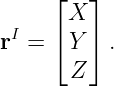
orbital-plane coordinates. With the argument of latitude u = ω + ν, the inertial Cartesian position
can be written
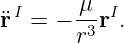
The inertial frame is useful because Newton’s two-body equation has its simplest form
there:
But a receiver antenna, a survey monument, and a point on Earth’s surface are naturally described
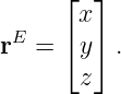
in a frame attached to the rotating Earth. That frame is Earth-centered, Earth-fixed, abbreviated
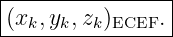
ECEF. Its Cartesian position is written
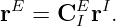
The next step in the navigation chain is therefore
The physics behind this step is simple: the Earth-fixed axes rotate relative to the inertial axes. The
bookkeeping is not simple, because a sign error in that rotation changes every satellite
longitude.
2 Idealized ECI and ECEF frames
For the present derivation, use an idealized pair of frames sharing the same origin at Earth’s center
and the same z axis. Let
be the inertial basis and
be the rotating Earth-fixed basis. In this simplified model,
The Earth-fixed x and y axes rotate eastward about the common z axis. Let 𝜃e(t) denote the angle
through which the Earth-fixed frame has rotated relative to the inertial frame.
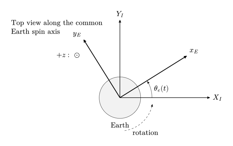
Figure 1. Idealized ECI and ECEF axes viewed along the common Earth spin axis.
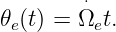
If the rotation rate is approximated as constant,
and therefore
For the legacy GPS broadcast equations the specified Earth rotation rate is
This is the value appearing in IS-GPS-200 broadcast user equations.
3 Active rotation versus coordinate transformation
A rotation matrix can be used in two logically different ways:
-
1.
- actively rotate a physical vector while the basis remains fixed;
-
2.
- keep the physical vector fixed while changing the basis in which its components are
reported.
ECI-to-ECEF is the second operation. The satellite does not jump when we change coordinate
frames. Only its components change.
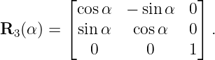
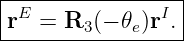
GPSORB08 used the active right-handed rotation
If the ECEF basis has actively rotated through +𝜃e, the coordinates of a fixed vector in that
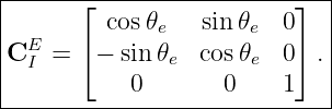
rotated basis are obtained with the inverse rotation:
Thus the inertial-to-Earth-fixed coordinate transformation matrix is
This sign pattern is also the R3 convention used in the Earth-orientation portion of
IS-GPS-200.
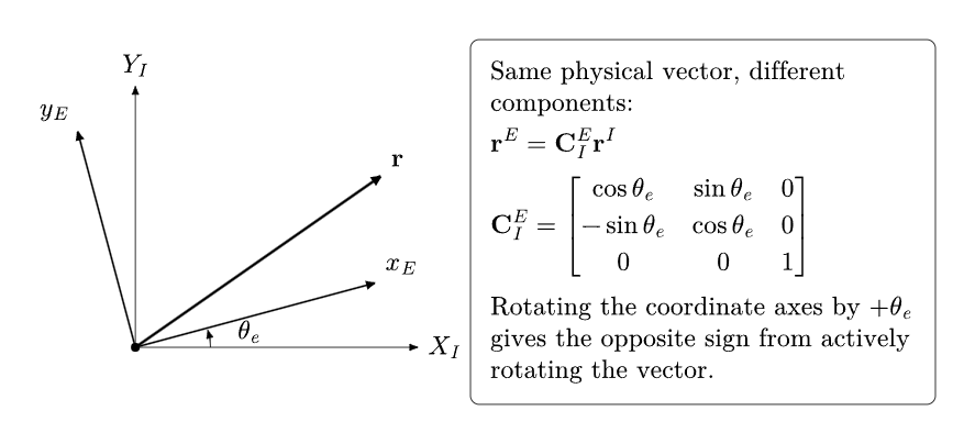
Figure 2. A fixed physical vector has different coordinate components in ECI and ECEF.
Equation (13) gives
Because CIE is orthogonal,
Therefore
4 A sign sanity check
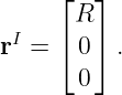
Suppose the ECI and ECEF frames coincide at t = 0. Place a fixed point on the positive inertial X
axis:
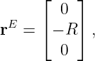
After Earth has rotated eastward by 90∘, the ECEF x axis points along inertial +Y . The
original inertial point therefore appears on the Earth-fixed negative y axis. Equation (13)
gives
which confirms the sign.
This is an extremely useful test in software. If the same thought experiment produces +R in the
Earth-fixed y component, the ECI-to-ECEF rotation sign has been reversed.
5 Differentiating the rotating-frame transformation
The position transformation contains time through 𝜃e(t). Consequently, velocity cannot be
transformed by applying only the same matrix to the inertial velocity.
Start with
Differentiate:
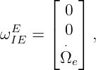
For a frame rotating with angular velocity
the derivative of the coordinate transformation satisfies
Hence
Equivalently,
This is the same transport-theorem physics that appears in strapdown navigation. Differentiating
once more, with constant Earth rate, produces the Coriolis and centrifugal terms
Those terms will reappear when the GPS broadcast acceleration equations are derived later in the
series.
6 The ascending node seen from two frames
The same frame-rotation geometry applies to the line of nodes. Let ΩI be the node angle measured
from the inertial reference direction, and let ΩE be the longitude of that same node measured from
the rotating ECEF x axis.
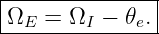
The geometry immediately gives
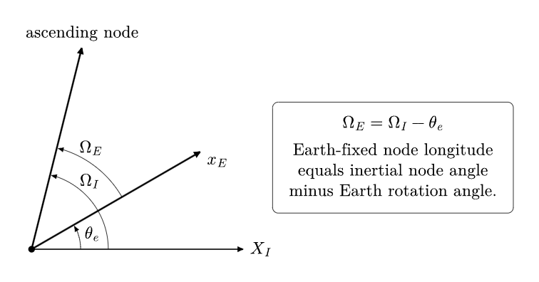
Figure 3. Earth-fixed node longitude is inertial node angle minus Earth rotation angle.
Equation (28) is the conceptual core of the GPS node-longitude equation. The satellite orbit plane
may itself precess slowly, while the Earth-fixed reference direction rotates rapidly underneath
it.
7 Allow the orbital plane to precess
In the ideal two-body problem,
A real GPS orbit experiences perturbations, especially from Earth’s oblateness, so the node drifts.
Over the relatively short broadcast-ephemeris fit interval, the GPS model represents that drift with
the broadcast rate  .
.
Let
be the elapsed time from the ephemeris reference epoch. In the GPS broadcast parameterization,
introduce the nonrotating-reference node angle
The superscript star is used here only to make the derivation transparent: Ω∗ is the node angle
before the Earth-fixed reference meridian is rotated away. It should not be interpreted
as a full modern celestial-frame right ascension. IS-GPS-200 formally names Ω0 the
“Longitude of Ascending Node of Orbit Plane at Weekly Epoch.” Because the broadcast
coefficients are curve-fit parameters, the normative meaning is the specified user equation as a
whole, not an attempt to reinterpret Ω0 as an independently propagated terrestrial
longitude.
Measure GPS time t from the beginning of the GPS week. In the simplified broadcast model the
accumulated Earth rotation is
Applying the same geometry as Eq. (28) to the broadcast angle gives
Since
Eq. (33) becomes
Collect the terms multiplying tk:
This is the longitude-of-ascending-node equation in IS-GPS-200 Table 20-IV and in Kaplan’s
broadcast-ephemeris position algorithm.
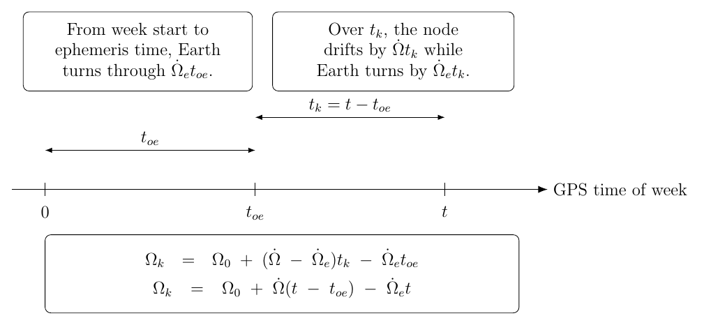
Figure 4. The GPS node equation separates week-start Earth rotation from propagation after the
ephemeris reference time.
8 Why the Earth-rate term seems to appear twice
Equation (36) contains both
and
There are not two different Earth rotations. Their sum is simply
The two terms appear because the GPS algorithm propagates the orbit using time measured from
toe while Earth orientation in the legacy formula is referenced to GPS time of week. The equation
must therefore account for Earth rotation from week start to toe and from toe to the evaluation
time.
The compact equivalent form is
The ICD form is preferred in implementation because it uses the already-computed quantity
tk.
9 The node rate in ECEF
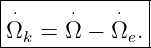
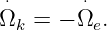
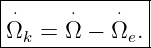
Differentiate Eq. (36). Since toe is fixed for a given ephemeris data set,
Therefore
This is exactly the node-rate expression used in the satellite-velocity portion of IS-GPS-200 Table
20-IV. It also gives a useful physical interpretation. Even if the orbital plane were perfectly fixed in
inertial space,
the Earth-fixed node longitude would still move at
The ground-fixed longitude of an inertially fixed orbital plane sweeps westward because Earth
rotates eastward beneath it.
10 Return to the orbital-plane coordinates
The broadcast algorithm does not ordinarily form an ECI position and then perform a separate
ECI-to-ECEF multiplication. Instead it folds the Earth rotation directly into the corrected node
longitude Ωk.
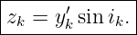
After computing corrected radius rk, argument of latitude uk, and inclination ik, define
These are coordinates in the orbital plane with the first axis along the ascending-node
direction.
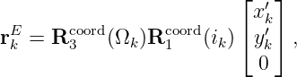
Rotating that in-plane vector by inclination and then by the Earth-fixed node longitude
gives
These are the Earth-fixed coordinate equations in the GPS broadcast user algorithm. Compare
them with GPSORB08: the algebraic structure is the same, but the angle multiplying the final
rotation is now Ωk, an Earth-fixed node longitude rather than a purely inertial right
ascension.
11 A matrix view of the same GPS equations
Equations (47)–(49) can be written compactly as
where the coordinate-transformation sign convention is chosen consistently with the component
equations above.
This is an important conceptual simplification:
Earth rotation does not require a separate correction after Eqs. (47)–(49); it is already embedded
in Ωk.
12 GPS time of week and week crossover
The quantity
looks harmless but needs careful implementation near the beginning or end of a GPS week. A GPS
week contains
IS-GPS-200 instructs the user to use the actual nearest time difference. Thus, after initially
computing tk,
and
Without this correction, an ephemeris valid across a week boundary can appear to be almost one
week old or one week in the future. The resulting errors in mean anomaly and node longitude
would be enormous.
The specification also defines t in the broadcast user equation as GPS system time at signal
transmission, with propagation time accounted for. This becomes important when a
receiver iterates satellite transmit time and applies Earth-rotation or Sagnac corrections
consistently.
13 Numerical example: corrected node longitude
Take the illustrative broadcast-like values
Then
The node’s inertial drift over the two-hour propagation interval is only
By comparison, Earth rotates during the same two hours through
Using Eq. (36),
This gives the unwrapped angle
Angles differing by integer multiples of 2π are equivalent, so wrapping to [0, 2π) gives
The example shows why Earth rotation dominates the node longitude over hour-scale intervals
even though the orbital plane’s inertial precession is physically important over longer
periods.
14 Numerical example: direct ECI-to-ECEF rotation
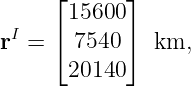
Consider the inertial position
and suppose the Earth rotation angle is
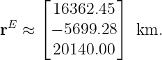
Equation (13) gives
The z component is unchanged because the idealized ECI and ECEF frames share their rotation
axis. The horizontal components change because the Earth-fixed axes have rotated beneath the
inertial vector.
15 What the simple Earth rotation model leaves out
The transformation
is intentionally simple. It is appropriate for understanding the legacy GPS broadcast position
equations, but it is not a complete high-precision transformation between a celestial reference
frame and a terrestrial reference frame.
At high precision, Earth orientation includes effects such as
- Earth rotation tied to UT1;
- precession and nutation of the Celestial Pole;
- polar motion;
- conventional celestial and terrestrial reference-frame realizations.
IS-GPS-200’s modern Earth-orientation material points users to the IERS Conventions for the
more complete inertial-to-geodetic transformation. The legacy broadcast orbit equations,
however, intentionally use the specified constant Earth rotation rate in the node-longitude
relation.
This distinction is important. One should not replace the broadcast user equation with an
arbitrary sidereal-time model and expect bit-for-bit agreement with a GPS receiver
implementation. Conversely, one should not use the simple legacy broadcast rotation as a
substitute for a precision ITRF/GCRF transformation in high-accuracy geodesy.
16 The chain from Newton to Earth-fixed GPS coordinates
The derivation sequence can now be summarized as
At this point the frame mechanics underlying Kaplan’s final position equations are no
longer a recipe: each Earth-fixed term follows from the geometry of a rotating coordinate
frame.
17 Summary
The main results are:
-
1.
- ECEF coordinates of a fixed physical vector are obtained from ECI coordinates by the
inverse of the active Earth rotation:
-
2.
- In the constant-rate model,
-
3.
- Node longitude in the rotating frame equals inertial node angle minus Earth rotation
angle:
-
4.
- With tk = t − toe, the GPS broadcast parameterization gives
-
5.
- The corresponding Earth-fixed node rate is
-
6.
- The final Earth-fixed position follows from
These equations form the frame-rotation bridge between classical orbital mechanics and the GPS
broadcast ECEF position algorithm.
References
References
[1] Global Positioning Systems Directorate, IS-GPS-200N: NAVSTAR GPS Space
Segment/Navigation User Interfaces, 1 August 2022, especially Tables 20-II and 20-IV.
[2] E. D. Kaplan and C. J. Hegarty, eds., Understanding GPS/GNSS: Principles and
Applications, 3rd ed., Artech House, 2017.
[3] O. Montenbruck and E. Gill, Satellite Orbits: Models, Methods, and Applications,
Springer, 2000.
[4] G. Petit and B. Luzum, eds., IERS Conventions (2010), IERS Technical Note No.
36, International Earth Rotation and Reference Systems Service, 2010.