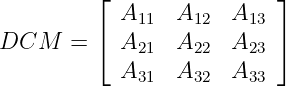
direction cosine matrix | Physics Library

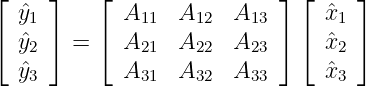
A direction cosine matrix (DCM) is a transformation matrix that transforms one coordinate reference frame to another. If we extend the concept of how the three dimensional direction cosines locate a vector, then the DCM locates three unit vectors that describe a coordinate reference frame. Using the notation in equation 1, we need to find the matrix elements that correspond to the correct transformation matrix.

⌊ ⌋ A11 A12 A13 DCM = ⌈ A21 A22 A23 ⌉ A31 A32 A33

(1)

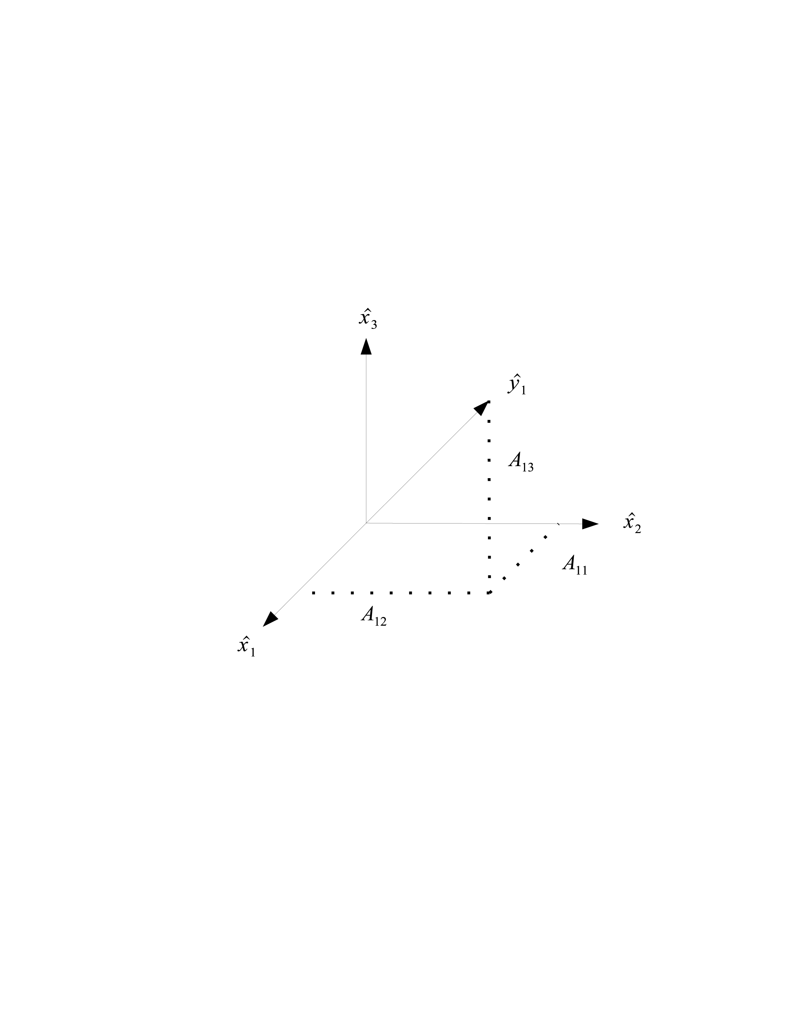
The first unit vector of the second coordinate frame can be located in the first frame by normal vector notation. See figure 1 for relationship.

ŷ₁ = A₁₁x₁ + A₁₂x₂ + A₁₃x₃

Similarily, the other two unit vectors can be described by

ˆy2 = A21xˆ1 + A22 ˆx2 + A23ˆx3

ˆy3 = A31xˆ1 + A32 ˆx2 + A33ˆx3

It is easy to see how equation 1 works as a transformation matrix through simple matrix multiplication.

⌊ ⌋ ⌊ ⌋ ⌊ ⌋ ˆy1 A11 A12 A13 ˆx1 ⌈ ˆy2 ⌉ = ⌈ A21 A22 A23 ⌉ ⌈ ˆx2 ⌉ ˆy3 A31 A32 A33 ˆx3

(2)

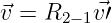
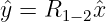
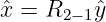
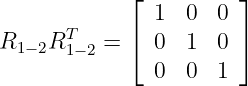
Once this transformation matrix is found, it can be used to transform vectors from the second frame to the first frame and vice versa. Equation 2 transforms the x frame to the y frame and can be denoted as R₁₋₂. In order to get R₂₋₁, which transforms the y frame to the x frame, we use a property of transformation matrices of orthonormal reference frames (a frame that is described by unit vectors and are perpindicular to each other). See the entry on a transformation matrix for more info on its properties. We use the properties that

− 1 T R1−2 = R 1−2 = R2− 1

⌊ ⌋ 1 0 0 R RT = ⌈ 0 1 0 ⌉ 1−2 1−2 0 0 1

so using these properties and rearranging equation 2

ˆy = R1− 2xˆ

yields

R −1−12ˆy = R−1−12R1 −2ˆx

giving the transformation of the y frame to the x frame

ˆx = R ˆy 2− 1

So to extend this concept to transform vectors from one frame to another a closer examination of a vector being represented in both frames is needed. If we denote the second frame as the prime (′) frame, then a vector expressed in each of these is given by

v = v1ˆx1 + v2ˆx2 + v3ˆx3

(3)

v = v1′ˆy1 + v2′ˆy2 + v3′yˆ3

(4)

Since both equations describe the same vector, let us set them equal to each other so

v1xˆ1 + v2ˆx2 + v3ˆx3 = v1′ˆy1 + v2′yˆ2 + v3′ˆy3

This notation is clumsy so we want to represent it in matrix notation. This is simple enough if you have an understanding of multiplying a column vector by a row vector. This allows us to describe equations 3 and 4 by

⌊ ⌋ ˆx1 v = [ v v v ]⌈ ˆx ⌉ 1 2 3 2 ˆx3

⌊ ⌋ ˆy1 v = [ v ′ v ′ v ′ ]⌈ ˆy ⌉ 1 2 3 2 ˆy3

Setting them equal and substituting equation 2 in for the second coordinate frame yields

⌊ ⌋ ⌊ ⌋ ⌊ ⌋ [ ] ˆx1 [ ] A11 A12 A13 ˆx1 v = v1 v2 v3 ⌈ ˆx2 ⌉ = v1′ v2′ v3′ ⌈ A21 A22 A23 ⌉ ⌈ ˆx2 ⌉ ˆx3 A31 A32 A33 ˆx3

Then by inspection (or go through the matrix manipulation to cancel the x frame)

⌊ ⌋ A11 A12 A13 [ v v v ] = [ v ′ v ′ v ′ ]⌈ A A A ⌉ 1 2 3 1 2 3 21 22 23 A31 A32 A33

Representing the transformation matrix as R₁₋₂ as the transformation from the first frame to the second frame and transposing the previous equation gives

[ ] [ ] T v1 v2 v3 = ( v1′ v2′ v3′ R1− 2)

Performing the transposition and using a transposition property for two matrices A and B such that

(AB )T = BT AT

leads to the relationship

⌊ v1 ⌋ ⌊ v1′⌋ ⌈ ⌉ T ⌈ ⌉ v2 = R 1−2 v2′ v3 v3′

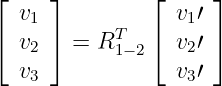
Finally giving us the ability to transform a vector from the second (prime) frame to the first frame.

⃗v = R2 −1⃗v′

Much much more can be found in the general entry about the Transformation matrix.

"direction cosine matrix" is owned by bloftin.
(view preamble)