|
|
|
|||||||
and the reciprocity result
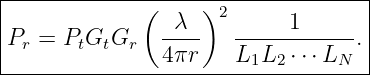
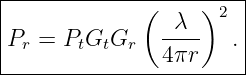
EM25 now combines those results with spherical electromagnetic power spreading to derive the Friis transmission equation, the free-space path-loss equation, and the logarithmic bookkeeping used in RF link budgets [1, 2, 3, 4]. The central derivation chain is
The result will be
under the assumptions developed below. This equation is often memorized. The purpose of this article is instead to make every factor physically visible.
1 Reference planes and assumptionsA link equation is only unambiguous when the power reference planes are stated. In the basic Friis derivation used here,
These assumptions will later be relaxed by adding explicit efficiency or loss factors.
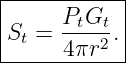
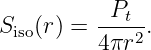
2 Step 1: directional transmitted powerFor an isotropic radiator with total power Pt, the power density at radius r is
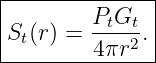
A real antenna redistributes the radiated power angularly. If its gain toward the receiver is Gt, then the far-field power density in that direction is
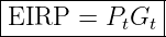
The numerator
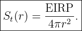
is the equivalent isotropically radiated power in that direction. Thus
The 1∕r2 dependence is geometric spreading. In ideal free space, power is not being converted to heat by this term. The same total outward power crosses larger and larger spherical surfaces.
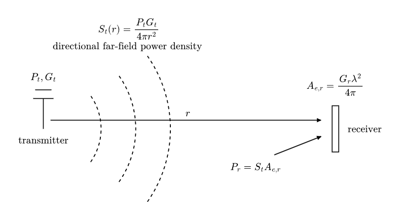
Figure. Friis geometry. Transmit gain sets the directional power density, spherical spreading produces the 1∕r2 factor, and the receiving antenna samples that power density through its effective aperture.
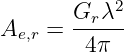
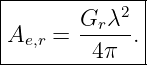
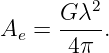
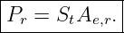
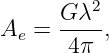
3 Step 2: receiving effective apertureEM24 defined effective aperture by
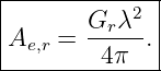
For a reciprocal receiving antenna with gain Gr,
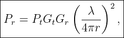
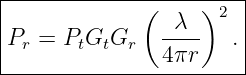
Substituting the transmitted power density gives
Therefore
This is the Friis transmission equation for the ideal free-space case [1].
4 What each Friis factor meansThe equation can be read as a sequence of physical transformations:
The factor
is therefore not an arbitrary communications-engineering correction. It appears because a transmitted wave spreads over an area proportional to r2, while an antenna of fixed receive gain has effective aperture proportional to λ2.
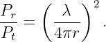
5 Free-space path lossFor isotropic antennas,
Then Friis becomes
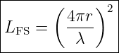
Define the dimensionless free-space path loss as the reciprocal power ratio,
Since
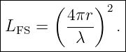
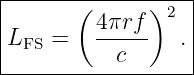
we may also write
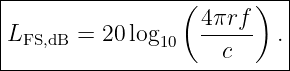
This is the free-space path-loss equation.
6 Free-space path loss is not dissipative attenuationThe word loss can be misleading. EM20 introduced material attenuation through an amplitude factor such as
where electromagnetic energy is transferred to the medium through dissipative mechanisms such as J ⋅ E. Free-space path loss is different. In ideal vacuum,
The power crossing a complete sphere remains constant, but the power density falls as
Thus free-space path loss describes the coupling between a finite receiving aperture and a geometrically expanding wavefront. It is not absorption by empty space.
7 The frequency dependence of path lossAt fixed antenna gains,
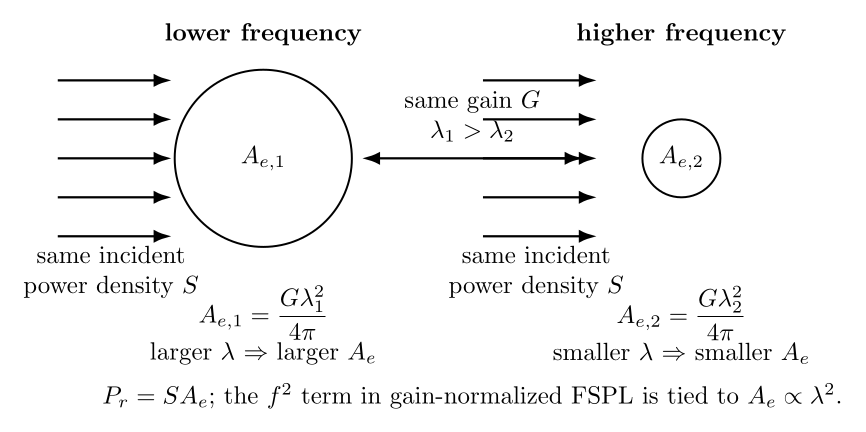
Therefore doubling frequency while keeping r, Gt, and Gr fixed increases free-space path loss by a factor of four. It is important to understand why. For fixed gain,
so higher frequency means smaller effective aperture. The geometric spreading term
contains no frequency. A wave of higher frequency does not geometrically “spread faster” in free space. The f2 dependence enters the gain-normalized Friis relation through the receive-aperture factor.
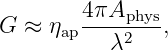
Figure. At the same incident power density and the same receive gain, effective aperture scales as λ2. The higher-frequency antenna therefore captures less power unless its gain is increased. For an aperture antenna of fixed physical area Aphys and fixed aperture efficiency,
so the gain increases as 1∕λ2. The frequency dependence of a complete link therefore depends on what physical quantities are being held fixed.
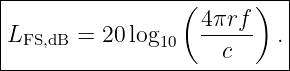
8 Decibel form of free-space path lossTaking 10 log 10 of the power ratio gives
Therefore
The factor of 20 appears because the underlying dimensionless ratio is squared before the logarithm is taken. Useful unit-specific forms follow from inserting the appropriate scale factors. With distance in kilometers and frequency in megahertz,
With distance in kilometers and frequency in gigahertz,
These constants are not new physics; they only encode the unit conversions and the factor 4π∕c.
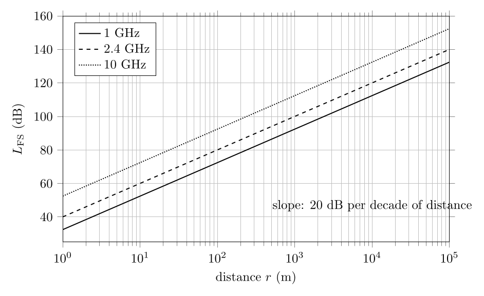
9 Scaling rules worth rememberingFrom the logarithmic form,
we obtain several immediate rules:
Figure. Free-space path loss versus distance at several frequencies. Each decade of distance adds 20 dB, while the vertical separation between curves reflects the 20 log 10f dependence at fixed antenna gains.
10 Example: an isotropic 2.4 GHz linkLet
with
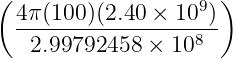
The free-space path loss is
Since
we obtain
In linear units,
11 Friis in decibel formFor the ideal link,
Taking logarithms gives
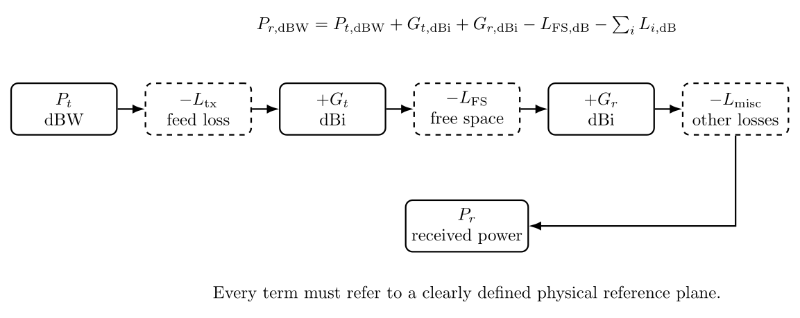
This additive form is the foundation of an RF link budget. The units should be tracked carefully:
Also,
12 Adding real link lossesLet Li ≥ 1 denote multiplicative power-loss factors. A generalized linear link may be written
In decibels,
Typical additional losses include
A clean link budget keeps each physical mechanism separate until there is a good reason to combine them.
Figure. A logarithmic link budget is conservation-style bookkeeping. Gains are added, losses are subtracted, and the result is the received power at a clearly defined reference plane.
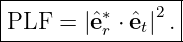
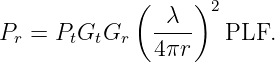
13 Polarization mismatchIf the incident and receiving polarization unit vectors are et and er, define the polarization loss factor
Then
The equivalent polarization loss in decibels is
For two linear polarizations separated by angle ψ,
At 45∘,
so the polarization loss is approximately
14 Impedance mismatch and realized gainIf the antenna terminal reflection coefficient is ΓA, the fraction of incident terminal power accepted by the antenna is
The corresponding mismatch loss is
If realized gain is used instead of ordinary gain, terminal mismatch is already incorporated. A link budget must not subtract the same mismatch twice. This is another reason reference-plane definitions are essential.
15 Example: a complete 5.8 GHz link budgetConsider an illustrative line-of-sight link with
The free-space path loss is
The EIRP after transmitter feed loss is
The final receive power is
Therefore
The important point is not this specific number. It is the auditable chain of reference planes and physical mechanisms that produced it.
16 Link marginIf a receiver requires at least Preq at the chosen reference plane, define the link margin as
A positive margin means the predicted receive power exceeds the stated requirement by that amount. At this stage Preq is simply an externally specified threshold. EM26 will replace this black-box threshold with receiver-noise physics: thermal noise, N0 = kT, noise temperature, noise figure, G∕T, and ultimately C∕N0.
17 Illustrative GNSS-like free-space linkTo prepare for that transition, consider an illustrative L-band link with
and directional transmit EIRP
For an ideal 0 dBi receiving antenna, the free-space path loss is
If all additional receive and propagation losses total 2 dB, then
Thus
This is an intentionally simplified GNSS-like example, not a specification for a particular satellite or receiver. Its purpose is to show why satellite-navigation signals arrive at very low power levels and why the next step must be a noise-density calculation rather than power alone.
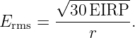
18 A second derivation using field strengthEM24 gave the free-space RMS electric field associated with EIRP,
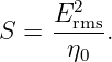
The corresponding incident power density is
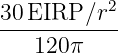
Using η0 ≈ 120π Ω,
Multiplying by
again gives Friis. This alternative route verifies that the link equation is consistent with the electromagnetic field-strength formulation.
19 Conditions for using FriisFriis is powerful because it compresses a field problem into a scalar power relation, but it is not universal. The standard form should be used only when its approximations are appropriate. Important checks include
20 Why the Friis factor can appear greater than one outside its domainThe isotropic free-space factor is
If one formally chooses a sufficiently small r, this factor can exceed one. That does not imply passive antennas create power. It means the far-field aperture model has been extrapolated outside the regime where it applies. Near-field energy exchange must be analyzed with the actual fields and mutual coupling, not with the far-field Friis equation.
21 From Friis to noise and interferenceEM25 has now completed the deterministic power-delivery chain
But received carrier power alone does not determine receiver performance. The next questions are
and later
The next stages of the series will therefore introduce
and eventually jammer-to-signal quantities such as J∕S.
22 SummaryA transmitting antenna with accepted power Pt and directional gain Gt produces far-field power density
A receiving antenna with gain Gr has effective aperture
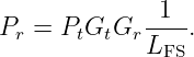
Multiplying the two yields Friis:
The corresponding free-space path loss is
or
A practical logarithmic link budget is then
The key physical distinction is that free-space path loss is geometric coupling loss, not dissipative attenuation of electromagnetic energy in vacuum.
References
References
[1] Harald T. Friis, “A Note on a Simple Transmission Formula,” Proceedings of the IRE, vol. 34, no. 5, pp. 254–256, 1946. [2] Constantine A. Balanis, Antenna Theory: Analysis and Design, 4th ed., Wiley, 2016. [3] Warren L. Stutzman and Gary A. Thiele, Antenna Theory and Design, 3rd ed., Wiley, 2012. [4] David M. Pozar, Microwave Engineering, 4th ed., Wiley, 2012. [5] IEEE, IEEE Standard for Definitions of Terms for Antennas, IEEE Std 145-2013, 2014. "Electromagnetic Waves, Antennas, and RF: Friis Transmission Equation, Free-Space Path Loss, and RF Link Budgets" is owned by bloftin.
Cross-references: power, relation, EM24 There are 12 references to this object. This is version 1 of Electromagnetic Waves, Antennas, and RF: Friis Transmission Equation, Free-Space Path Loss, and RF Link Budgets, born on 2026-10-10. Object id is 1455, canonical name is ElectromagneticWavesAntennasAndRFFriisTransmissionEquationFreeSpacePathLossAndRFLinkBudgets. Accessed 10 times total. Classification:
|
|
|
|
Pending Errata and AddendaNone.
|
DiscussionNo messages.
|
Interact |











![[ ]
( 4πr )2
----
λ](https://images.physicslibrary.org/cache/objects/1455/make4ht/ElectromagneticWavesAntennasAndRFFriisTransmissionEquationFreeSpacePathLossAndRFLinkBudgets28x.png)