|
|
|
|||||||
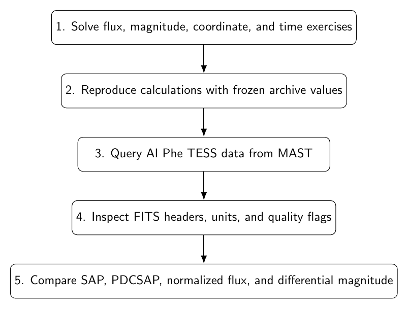
Figure 1. The BIN02E1 workflow moves from unit-aware calculations to frozen archive values, then to live public data and FITS inspection.
Part I: Problems
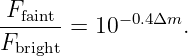
Problem 1: magnitude difference to flux ratioTwo binary components differ by
magnitudes in the same passband. Find
Problem 2: combined magnitudeTwo unresolved components have magnitudes
Find the combined magnitude.
Problem 3: equal-component binaryShow that an unresolved pair of equal-flux stars is approximately 0.7526 magnitude brighter than either component alone.
Problem 4: eclipse depthA normalized Light curve falls from
to
Find:
Problem 5: color indexA catalog gives
Find the Gaia color
Problem 6: small-angle separationTwo resolved components have coordinate differences
at mean declination
Estimate their angular separation.
Problem 7: position angleUsing the offsets from Problem 6, find the approximate position angle measured from north through east.
Problem 8: MJD conversionConvert
to JD.
Problem 9: TESS time conversionA TESS sample has
Convert to full
Problem 10: magnitude uncertaintyA flux measurement has
Estimate the magnitude uncertainty in the small-error approximation.
Problem 11: spectral resolutionA spectrograph operates at
Estimate:
Problem 12: third-light dilutionA binary would have an intrinsic fractional eclipse depth
relative to the binary’s own out-of-eclipse flux. An unrelated source contributes
of the binary’s out-of-eclipse flux. Find the observed eclipse depth.
Part II: Complete worked solutions
Solution 1Use
Therefore
The brighter star provides ten times the flux of the fainter star in that passband.
Solution 2Convert each magnitude to relative flux:
The total relative flux is
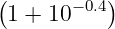
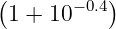
Factor out 10−3.2:
Thus
The unresolved system is brighter than either component.
Solution 3For equal component flux F,
Therefore
Hence
Solution 4The fractional depth is
The differential magnitude is
Solution 5
Solution 6The east-west tangent-plane offset is
The north-south offset is
Therefore
Solution 7Measured from north through east,
Solution 8By definition,
Therefore
Solution 9Using
Solution 10
Therefore
Solution 11The wavelength resolution is
Using
Solution 12Let the binary out-of-eclipse flux be
The contaminating flux is
The intrinsic eclipse removes
The observed out-of-eclipse flux is
Therefore
Third light has diluted a 40% intrinsic eclipse to about 33.3% in the observed aperture.
Part III: Frozen archive exercisesThe file BIN02E1_frozen_photometry.csv
It preserves a small educational snapshot of public photometric values used in this sequence. The file includes bright-system values from the SIMBAD snapshot already introduced in BIN01 and a separate AI Phe metadata file for the TESS data lab.
Exercise A: Algol flux ratiosUsing the frozen Algol values
compute
and compare the relative B- and V -band fluxes using the magnitude relation. Do not interpret the result as a pure temperature measurement without considering
Exercise B: Sirius versus Algol in VThe frozen snapshot gives approximately
The magnitude difference is
Therefore the ratio of their observed V -band fluxes is
This is an observed flux ratio at Earth, not a luminosity ratio.
Part IV: TESS/MAST data lab with AI PhoenicisAI Phoenicis is a bright detached eclipsing binary observed by TESS. The frozen metadata file BIN02E1_AI_Phe_TESS_metadata.csv
records the observational facts needed to reproduce the introductory lab. The important identifiers are
Published analyses of these data report that TESS observed AI Phe in Sector 2 with two-minute cadence and that the sector covered both primary and secondary eclipse.
Figure 2. The AI Phe lab queries MAST, selects the Sector 2 TESS light curve, inspects FITS metadata, applies an explicit quality rule, and compares SAP with PDCSAP photometry.
Lab 1: live archive searchThe supplied Python script uses lightkurve to search MAST: search = lk.search_lightcurve( "AI Phe", mission="TESS", sector=2 )
Record:
Lab 2: inspect the light curveDownload one standard SPOC light-curve product. Inspect
Do not begin by plotting only the default flux column. First determine what that column represents.
Lab 3: quality maskingCreate a strict introductory mask using
Then compare the number of retained and rejected samples. This is intentionally simple. Later methods articles can adopt mission bitmasks tailored to a specific scientific question.
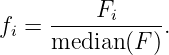
Lab 4: normalized fluxFor the retained PDCSAP samples, define
Plot
against BTJD. Identify the primary and secondary eclipse.
Lab 5: differential magnitudesConvert the normalized flux to
Verify that
Lab 6: SAP versus PDCSAPPlot normalized SAP and PDCSAP flux on the same time interval. Ask:
The correct lesson is not that one column is universally superior. The lesson is that pipeline processing choices are part of the measurement model.
Part V: FITS inspectionIf the downloaded light curve is available locally, inspect it with from astropy.io import fits with fits.open(filename) as hdul: hdul.info() print(hdul[0].header) print(hdul[1].header) print(hdul[1].columns)
Record at least:
A FITS light curve is not merely an array of numbers. The header provides the context necessary to interpret those numbers.
Part VI: What should be savedA reproducible submission for this lab should save:
Data-provenance noteThe AI Phe metadata shipped with this lesson is a small frozen record assembled from the published TESS analysis of AI Phe and public mission documentation. The frozen file is not a replacement for the MAST light-curve file. Students should rerun the live query whenever network access is available and compare the returned metadata with the frozen record.
SummaryThis companion establishes five operational habits:
These habits will be reused throughout the entire BIN series.
References
References
[1] B. W. Carroll and D. A. Ostlie, An Introduction to Modern Astrophysics, 2nd ed., Cambridge University Press, 2017. [2] ESA and Gaia DPAC, Gaia Data Release 3 Documentation, Gaia Archive Data Model, release 1.3, 2023. [3] P. F. L. Maxted et al., The TESS Light Curve of AI Phoenicis, Monthly Notices of the Royal Astronomical Society, 498, 332–343, 2020. [4] G. R. Ricker et al., Transiting Exoplanet Survey Satellite, Journal of Astronomical Telescopes, Instruments, and Systems, 1, 014003, 2015. [5] Astropy Collaboration, The Astropy Project, Astrophysical Journal, 935, 167, 2022. "Flux, Magnitudes, Coordinates, Time, and FITS" is owned by bloftin.
This object's parent. Cross-references: type, units, parameter, eclipsing binary, luminosity, calibration, temperature, relation, Algol, BIN01, system, velocity, flux, position, declination, color, Light, magnitudes, BIN02 This is version 1 of Flux, Magnitudes, Coordinates, Time, and FITS, born on 2026-10-06. Object id is 1427, canonical name is FluxMagnitudesCoordinatesTimeAndFITS. Accessed 4 times total. Classification:
|
|
|
|
Pending Errata and AddendaNone.
|
DiscussionNo messages.
|
Interact |
![[parent]](https://images.physicslibrary.org/images/uparrow.png)