1. Introduction

Boundary-value problems for the differential equations of the theory of elasticity have in common with many other differential-equation problems the property of being equivalent to problems of the calculus of variations. Recognition of this fact, for the problems of the elastic rod, goes back to Euler and Daniel Bernoulli. The general three-dimensional problem was first considered in this fashion by Green, in 1837.

We may, in the discussion of variational principles in elasticity, distinguish a number of phases as follows:

1. The formulation of different variational principles and their interrelation. The best-known examples of this are Green’s minimum principle for displacements and Castigliano’s maximum principle for stresses.
2. The application of variational principles to the establishment of approximate two- and one-dimensional theories for three-dimensional problems. A classical example of this is Kirchhoff’s treatment of the differential equations and boundary conditions for transverse bending of thin plates.
3. The application of variational principles for the determination of numerical values of the solution of boundary-value problems.
4. The simultaneous use of different variational principles for the determination of upper and lower bounds of numerical values.
5. The use of variational principles for the proof of uniqueness and existence theorems in elasticity theory.

The present paper has as its object the consideration of some of the questions associated with phases 1 and 4, as they have been of interest to the author.

2. The boundary-value problem

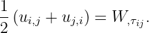
We consider the following system of nine differential equations for six components of stress, τ_ij = τ_ji, and three components of displacement, u_i:

(1)

(2)

In these equations and in what follows we make use of the summation convention according to which one sums over repeated subscripts. A comma in front of a subscript denotes partial differentiation with respect to the variable in question, except that f_,i indicates differentiation of f with respect to the Cartesian coordinate x_i.

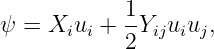
The function ψ in the equilibrium equations is taken in the form

(3)

where the X_i and Y _ij = Y _ji are given functions of the coordinates x_i.

The function W in the stress-strain relations (2) is taken in the form

(4)

where the A_ij = A_ji and B_ijkl = B_jikl = B_ijlk = B_jilk are given functions of x_i.

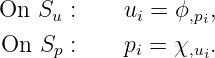
The system (1) and (2) is to be solved in the interior of a region V with boundary surface S. We divide the surface S in two parts, S_u and S_p, and consider the following system of conditions:

(5)

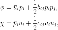
The functions ϕ and χ are taken in the form

(6)

where ū_i, p_i, b_ij = b_ji, and c_ij = c_ji are given functions of position on S_u and S_p, respectively. The quantities p_i are the x_i-components of the surface-stress intensity, given by

(7)

where n is the outward normal direction to the surface S.

The system of equations (1), (2), and (5), with ψ, W, ϕ, and χ defined by (3), (4), and (6), may be shown to represent the Euler equations and natural boundary conditions of a variational problem as stated below.

3. The general variational equation

Appropriate synthesis leads to the conclusion that a variational problem which has the differential equations (1) and (2) as Euler (differential) equations and the boundary conditions (5) as natural (or Euler) boundary conditions is the problem

(8)

where

(9)

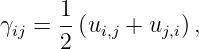
the quantities γ_ij being defined by

(10)

and where the τ_ij and u_i are varied independently. A related variational theorem in which (10) is not used merely as a definition, but is included among a system of equations for stresses, strains, and displacements, was formulated by K. Washizu in 1955 [2].

To verify the correctness of the above statement, we write

δI =	∫ V dV
	−∫ Spχ,ui δui dS −∫ Su dS.	(11)

We transform the second term in the volume integral by integration by parts:

(12)

Combination of (11) and (12) gives

δI =	∫ V dV
	+ ∫ Sp δui dS −∫ Su δpi dS,	(13)

and this shows that the Euler equations of the problem are the differential equations (1) and (2) and the boundary conditions (5).

The variational theorem implied by (8)–(10) is a generalization of a theorem which was formulated earlier [3]. It reduces to the earlier theorem if it is assumed that the body-force function ψ is absent and that the functions ϕ and χ in the boundary conditions are of the form

(6′)

What we have done in going from (6′) to (6) is to take the step from having either stress or displacement boundary conditions on S_p and S_u to a system of mixed boundary conditions on both S_p and S_u in such a manner as to preserve the form of the original theorem as a special case. Were it not for the desirability of accomplishing this within the framework of the generalized problem, there would, for the generalized problem, be no need for a separate consideration of the boundary portions S_p and S_u.

4. Variational equations for displacements or stresses

In order to bring out the significance of the general variational equation (8) for displacements and stresses, we state separately the less-general variational equations for displacements or stresses. In doing this, we are limiting ourselves here to stress and displacement boundary conditions of the form (6′).

a. Variational principle for displacements (Green)

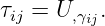
The stress-strain relations (2) are considered as equations of definition for the stresses (so that stress variations are dependent on displacement variations), and displacement variations are limited such that δu_i = 0 on S_u. Equations (2) are inverted and written, with the help of a function U, in the form

(14)

We further find that

(15)

and that the variational equation which has the equilibrium equations (1) and the stress boundary conditions in (6′) as Euler equations is of the form

(16)

where

(17)

b. Variational principle for stresses (Castigliano)

We now assume that stress variations and displacement variations are such that all comparison states are equilibrium states. We then have δp_i = 0 on S_p and

(18)

in the interior of the body.

We find that the variational equation which has the stress-strain relations (2) and the displacement boundary conditions in (6′) as Euler equations is of the form

(19)

where

(20)

We may note that, as long as ψ is a linear function of the u_i, which corresponds to the case of body forces independent of displacements, we have ψ − u_iψ_,ui = 0 and therewith the disappearance of body-force terms in the variational equation. The extension of the principle to the case where ψ is a special quadratic function of the u_i, which allows use of the principle in connection with vibration problems, has been stated previously [4].

5. A transformation and two inequalities

Useful information may be deduced from a comparison of the values of I for functions τ_ij and u_i which are not solutions of δI = 0 and for the functions τ_ij and u_i which are determined from δI = 0. We may designate the solution functions of δI = 0 by τ_ij and u_i and write

(21)

If we introduce (21) in (9), we shall have

I =	∫ V (γij + δγij)(τij + δτij) − ψ(u + δu) − W(τ + δτ)dV
	−∫ Spχ(u + δu) dS
	−∫ Su(pi + δpi)(ui + δui) − ϕ(p + δp)dS.	(22)

We shall from now on in this section limit ourselves to the case for which ψ, χ, and ϕ are linear functions and W is a homogeneous second-degree function. We then have

ψ(u + δu)	= Xiui + Xiδui,	(23a)
χ(u + δu)	= piui + piδui,	(23b)
ϕ(p + δp)	= uipi + uiδpi,	(23c)

and

(24)

We further write

(25)

where I is the value of I when τ_ij = τ_ij and u_i = u_i, where δI contains all terms linear in the variations δτ_ij and δu_i, and where δ²I contains all terms of second degree in the variations. Rearrangement of terms in (22) gives us

I =	∫ V dV −∫ Sppiui dS
	−∫ Su(ui −ūi)pi dS,	(26)

(27)

as it should be, and

(28)

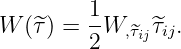
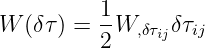
Equations (26) and (28) may be simplified if account is taken of some of the basic relations. Since W is homogeneous of the second degree, we have

(29)

Furthermore, γ_ij = W_,τij, while u_i = ū_i on S_u, and p_i = p_i on S_p. Therewith

(30)

We further have

(31)

and, since τ_ij,j + X_i = 0, finally

(32)

In order to transform δ²I as given by (28), we have at our disposal the relations

(33)

and

(34)

It is not immediately apparent in which way to utilize these two facts. However, let us write δ²I in the following two alternate forms:

(35)

or

(36)

In general, the quantity δ²I may be made both positive and negative by a suitable choice of the integrands. There are two exceptional cases where this is not so. These cases are given when

(37)

or when

(38)

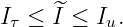
We now take account of the fact that the function W is positive-definite. Accordingly, when (37) holds, we have δ²I ≤ 0, and when (38) holds, we have 0 ≤ δ²I. We note that (37) represents the same limitations on variations as those associated with the variational principle for stresses [equation (19)] and that (38) represents the same limitations on variations as those associated with the variational principle for displacements [equation (16)]. We conclude then from (25) and (27) that the following basic inequality holds:

(39)

Equation (39) confirms the known fact that, in the variational theorem for displacements, one is concerned with a minimum problem and, in the variational theorem for stresses, one is concerned with a maximum problem. In contrast to this, the general variational theorem for stresses and displacements is no more than a stationary-value problem.

What is of importance in the present demonstration of this known fact is the explicit way in which both the minimum principle for displacements and the maximum principle for stresses are seen to be direct consequences of a more general principle for stresses and displacements.

Massachusetts Institute of Technology, Cambridge, mass.

Source note

This PhysicsLibrary entry is a conversion of the public-domain material in Reference [1].

References