Electromagnetic Waves, Antennas, and RF: Electromagnetic Energy, Poynting Vector, and
Intensity - Exercises and Complete Worked Solutions
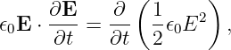
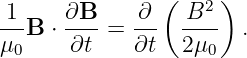
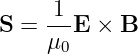
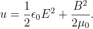
EM17 introduced electromagnetic energy density, the Poynting vector, Poynting’s theorem,
plane-wave intensity, vacuum impedance, and spherical spreading. This companion article turns
those ideas into a sequence of worked problems. The emphasis is on connecting the field quantities
E and B to measurable energy, power, and intensity while keeping the local conservation law
visible throughout the calculations.
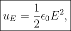
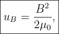
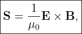
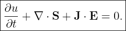
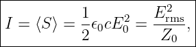
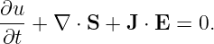
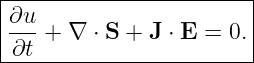
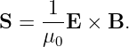
The central relations are
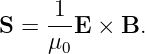
and
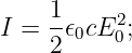
For a sinusoidal plane wave in vacuum,
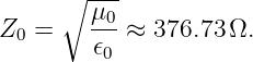
where
These formulas are most useful when treated as consequences of electromagnetic energy
conservation rather than as isolated expressions [1, 2, 3, 4, 5].
How to use this problem set
Attempt all exercises in Part I before consulting Part II. For each problem, first identify whether
the requested quantity is an energy density, an energy flux, a total power, or a time average. This
avoids one of the most common mistakes in this topic: mixing quantities with units of J/m3,
W/m2, and W.
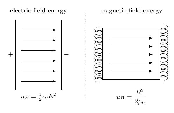
Figure. Electric and magnetic field energy densities have different field dependences but
the same units of J/m3.
Part I: Exercises
Exercise 1: electric-field energy density from a capacitor
A vacuum parallel-plate capacitor has
Neglect fringing. Find:
- the capacitance;
- the stored electrostatic energy from UE = CV 2∕2;
- the Electric Field magnitude;
- the field energy density uE;
- the total energy obtained by multiplying uE by the field-filled volume Ad.
Use the result to verify explicitly that the lumped-element and field-energy descriptions
agree.
Exercise 2: magnetic-field energy density from a solenoid
An ideal vacuum solenoid has
Find:
- the inductance L;
- the magnetic field magnitude inside the solenoid;
- the magnetic energy density uB;
- the total field energy uBAℓ;
- the inductive energy LI2∕2.
Verify that the two energy calculations agree.
Exercise 3: equal electric and magnetic energy in a vacuum plane wave
A vacuum plane wave has instantaneous electric-field magnitude E = 75 V/m at some point and
time.
Using
calculate:
- B;
- uE;
- uB;
- the total instantaneous electromagnetic energy density u.
Show numerically that uE = uB.
Exercise 4: direction and magnitude of the Poynting vector
At a point in vacuum,
and
Find the instantaneous Poynting vector
State both its magnitude and direction. Then compare B with the plane-wave value
E∕c.
Exercise 5: average intensity of a sinusoidal plane wave
A sinusoidal vacuum plane wave has peak electric-field amplitude
Find:
- the peak magnetic-field amplitude B0;
- Erms and Brms;
- the time-averaged intensity using
- the same intensity using
Exercise 6: infer field amplitudes from measured intensity
A receiver measures an average electromagnetic intensity
for a nearly plane vacuum wave.
Find:
- Erms;
- E0;
- Brms;
- B0.
Exercise 7: power through a tilted receiving surface
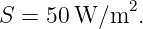
A uniform time-averaged Poynting vector has magnitude
It crosses a flat receiver of area
The receiver’s outward area normal makes an angle
with the direction of S.
Find the magnitude of the electromagnetic power crossing the surface. Explain why the cosine uses
the angle to the surface normal, not the angle to the surface itself.
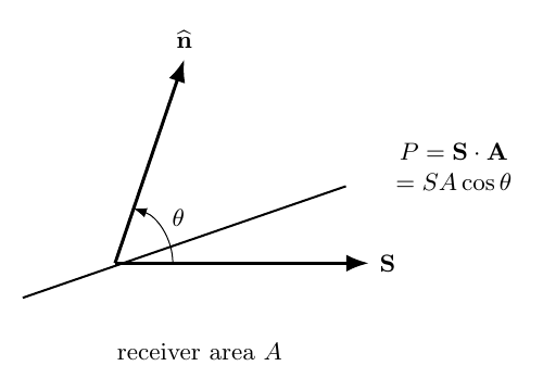
Figure. Power through a flat surface is determined by the projection S ⋅ A = SA cos 𝜃,
where 𝜃 is measured from the area normal.
Exercise 8: integral Poynting theorem and energy bookkeeping
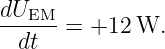
Inside a fixed control volume, the electromagnetic field energy is increasing at the rate
At the same time, the fields transfer energy to matter inside the volume at the rate
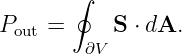
Using the integral form of Poynting’s theorem,
find the net outward electromagnetic power through the boundary. Interpret the sign
physically.
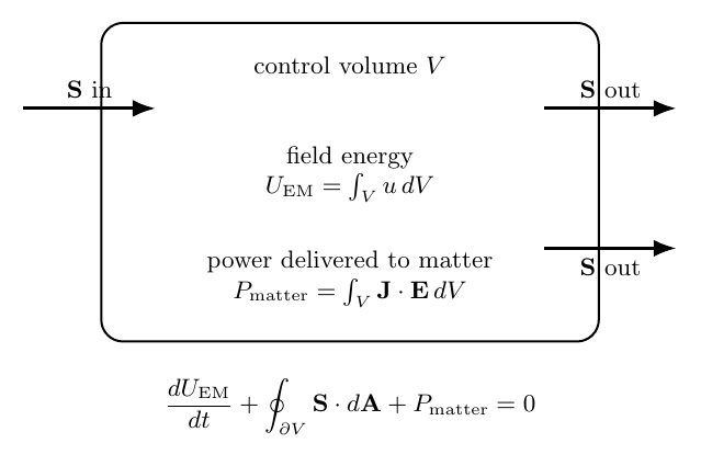
Figure. Poynting’s theorem balances field-energy accumulation, electromagnetic flux
through the boundary, and energy transfer from fields to matter.
Exercise 9: local Joule heating from J ⋅ E
Within a small conducting region, the fields and current density are approximately
uniform:
The Conductor volume is
Find:
- the local electromagnetic power-transfer density J ⋅ E;
- the total power transferred from the fields to the material in this volume;
- the result if the current density were reversed while E remained unchanged.
Interpret the sign of J ⋅ E.
Exercise 10: derive Poynting’s theorem from Maxwell’s equations
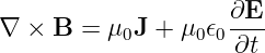
Starting with
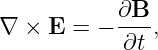
and
perform the following steps:
- dot the first equation with E∕μ0;
- dot the second equation with B∕μ0;
- combine the results using
- identify the time derivatives of uE and uB;
- derive
State the physical meaning of each term.
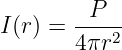
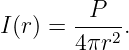
Exercise 11: spherical spreading and the difference between power and amplitude
An isotropic radiator emits total power
Assume lossless far-field propagation.
Find the intensity at
and
Then determine:
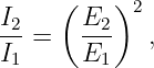
- the intensity ratio I2∕I1;
- the electric-field amplitude ratio E2∕E1;
- the magnetic-field amplitude ratio B2∕B1.
Explain why power density follows 1∕r2 while field amplitude follows 1∕r.
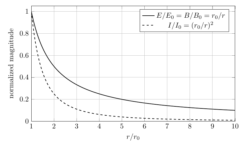
Figure. In lossless spherical far-field spreading, intensity falls as 1∕r2, while the electric-
and magnetic-field amplitudes fall as 1∕r.
Exercise 12: transmitter gain, power density, and received field strength
A transmitter radiates
through an antenna with gain
in the direction of a receiver 100 m away. Treat G as a linear power ratio and assume far-field
free-space propagation.
Find:
- the equivalent isotropically radiated power PtG;
- the intensity at the receiver;
- Erms;
- the peak electric-field amplitude E0.
Exercise 13: why power uses 10 log 10 but field amplitude uses 20 log 10
For a plane wave in a fixed medium,
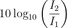
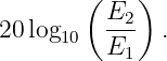
Show that the intensity ratio in decibels can be written either as
or as
Then evaluate both expressions when the distance from an ideal spherical radiator doubles. Show
that they give the same decibel change.
Exercise 14: standing waves can store energy without carrying net average power
Two equal-amplitude plane waves travel in opposite directions along z with the same polarization.
Their superposition is
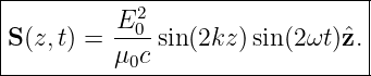
Find the instantaneous Poynting vector. Then show that its time average over one period is zero
everywhere. Explain how this is consistent with the fields possessing nonzero electromagnetic
energy.
Exercise 15: electromagnetic energy carried by a finite pulse
A plane electromagnetic pulse in vacuum has uniform cross-sectional area
and duration
During the pulse, approximate its average intensity as constant at
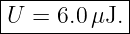
Find:
- the average power transported through the cross section;
- the total electromagnetic energy carried by the pulse;
- the spatial pulse length L = cΔt;
- the pulse volume AL;
- the average electromagnetic energy density obtained from U∕(AL);
- verify that this equals I∕c.
Exercise 16: Julia check of inverse-square and inverse-distance scaling
Write a short Julia program that evaluates, for 1 ≤ r ≤ 100 m,
and
for an isotropic radiator with P = 1 W.
Use logarithms to estimate the slopes of I(r) and Erms(r) versus r on log-log axes. The expected
slopes are −2 and −1, respectively.
Part II: Complete Worked Solutions
Solution 1: electric-field energy density from a capacitor
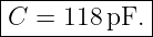
The capacitance is
| C | = 𝜖0 | (41)
|
| = (8.854 × 10⁻¹²)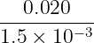 | (42)
|
| = 1.18 × 10⁻¹⁰ F. | (43) |
Thus,
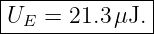
The stored energy is
| UE | =  CV 2 CV 2 | (45)
|
| =  (1.18 × 10⁻¹⁰)(600)2 (1.18 × 10⁻¹⁰)(600)2 | (46)
|
| = 2.13 × 10⁻⁵ J. | (47) |
Therefore,
The electric field is
| E | =  | (49)
|
| = 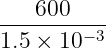 | (50)
|
| = 4.00 × 10⁵ V/m. | (51) |
The electric energy density is
| uE | =  𝜖0E2 𝜖0E2 | (52)
|
| =  (8.854 × 10⁻¹²)(4.00 × 10⁵)2 (8.854 × 10⁻¹²)(4.00 × 10⁵)2 | (53)
|
| = 0.708 J/m3. | (54) |
The field-filled volume is
Hence
| uEAd | = (0.708)(3.0 × 10⁻⁵) | (56)
|
| = 2.13 × 10⁻⁵ J. | (57) |
This agrees with CV 2∕2, confirming that the capacitor energy may be regarded as energy stored in
the electric field.
Solution 2: magnetic-field energy density from a solenoid
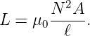
For an ideal long solenoid,
Thus,
| L | = (1.2566 × 10⁻⁶)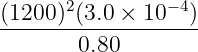 | (59)
|
| = 6.79 × 10⁻⁴ H. | (60) |
Therefore,
The magnetic field is
| B | = μ0 I I | (62)
|
| = (1.2566 × 10⁻⁶) (2.0) (2.0) | (63)
|
| = 3.77 × 10⁻³ T. | (64) |
The magnetic energy density is
| uB | =  | (65)
|
| = 5.65 J/m3. | (66) |
The field volume is
Hence
| uBAℓ | = (5.65)(2.40 × 10⁻⁴) | (68)
|
| = 1.36 × 10⁻³ J. | (69) |
The inductive energy is
 LI2 LI2 | =  (6.79 × 10⁻⁴)(2.0)2 (6.79 × 10⁻⁴)(2.0)2 | (70)
|
| = 1.36 × 10⁻³ J. | (71) |
Thus the field and lumped-element pictures agree.
Solution 3: equal electric and magnetic energy in a vacuum plane wave
The magnetic field is
| B | =  | (72)
|
| = 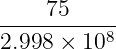 | (73)
|
| = 2.50 × 10⁻⁷ T. | (74) |
The electric energy density is
| uE | =  𝜖0E2 𝜖0E2 | (75)
|
| =  (8.854 × 10⁻¹²)(75)2 (8.854 × 10⁻¹²)(75)2 | (76)
|
| = 2.49 × 10⁻⁸ J/m3. | (77) |
For the magnetic energy density,
| uB | =  | (78)
|
| = 2.49 × 10⁻⁸ J/m3. | (79) |
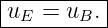
Thus
The total energy density is
This equality follows generally for a vacuum plane wave because B = E∕c and c−2 = μ
0𝜖0.
Solution 4: direction and magnitude of the Poynting vector
The cross product is
Since
we obtain
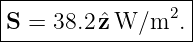
| S | =  (4.80 × 10⁻⁵)z (4.80 × 10⁻⁵)z | (84)
|
| = 38.2 z W/m2. | (85) |
Therefore,
The plane-wave prediction is
 | = 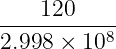 | (87)
|
| = 4.00 × 10⁻⁷ T, | (88) |
which matches the specified B to the shown precision. The fields are therefore consistent with an
instantaneous sample of a plane wave propagating in the +z direction.
Solution 5: average intensity of a sinusoidal plane wave
The peak magnetic amplitude is
| B0 | =  | (89)
|
| = 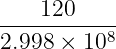 | (90)
|
| = 4.00 × 10⁻⁷ T. | (91) |
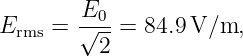
The RMS amplitudes are
and
Using the peak-field expression,
| I | =  𝜖0cE02 𝜖0cE02 | (94)
|
| =  (8.854 × 10⁻¹²)(2.998 × 10⁸)(120)2 (8.854 × 10⁻¹²)(2.998 × 10⁸)(120)2 | (95)
|
| = 19.1 W/m2. | (96) |
Using the RMS form,
| I | =  | (97)
|
| =  | (98)
|
| = 19.1 W/m2. | (99) |
Both methods agree.
Solution 6: infer field amplitudes from measured intensity
From
we obtain
| Erms | =  | (101)
|
| =  | (102)
|
| = 30.7 V/m. | (103) |
Therefore,
The magnetic fields follow from B = E∕c:
Solution 7: power through a tilted receiving surface
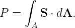
The power crossing a surface is
For uniform S over a flat area,
Hence
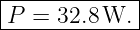
| P | = (50)(0.80) cos 35∘ | (109)
|
| = 32.8 W. | (110) |
Therefore,
The dot product uses the area vector A = An, so the relevant angle is the angle between S and the
surface normal. If an angle to the plane itself is given, it must first be converted to its
complementary angle relative to the normal.
Solution 8: integral Poynting theorem and energy bookkeeping
Write
Poynting’s theorem gives
Therefore,
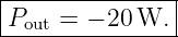
A negative outward flux means that the net electromagnetic flux is actually inward. Twenty watts
of electromagnetic power enters the volume. Of that incoming power, 12 W increases stored field
energy and 8 W is transferred to matter:
This is precisely the energy balance encoded by the sign convention in Poynting’s theorem.
Solution 9: local Joule heating from J ⋅ E
Because J and E are parallel,
| J ⋅ E | = (3.0 × 10⁶)(0.050) | (116)
|
| = 1.50 × 10⁵ W/m3. | (117) |
Thus,
The total material power is
| Pmatter | = (J ⋅ E)V | (119)
|
| = (1.50 × 10⁵)(2.0 × 10⁻⁵) | (120)
|
| = 3.0 W. | (121) |
If the current density is reversed,
The negative sign means that, locally, matter is transferring energy to the electromagnetic field
instead of receiving energy from it. Positive J ⋅ E corresponds to field energy being delivered to
charges, as in ordinary Joule heating.
Solution 10: derive Poynting’s theorem from Maxwell’s equations
Start from the Ampere–Maxwell law:
Dot with E∕μ0:
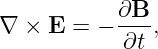
Now begin with Faraday’s law,
and dot with B∕μ0:
Use the Vector Identity
Substituting the two Maxwell relations gives
Recognize
and
Define
and
Then
The three terms mean, respectively: local accumulation of electromagnetic field energy, net
outward electromagnetic energy flux, and local transfer of electromagnetic energy to
matter.
Solution 11: spherical spreading and the difference between power and amplitude
For an isotropic radiator,
At r1 = 2.0 m,
| I1 | =  | (135)
|
| = 1.99 × 10⁻¹ W/m2. | (136) |
At r2 = 20 m,
| I2 | =  | (137)
|
| = 1.99 × 10⁻³ W/m2. | (138) |
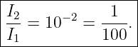
Therefore,
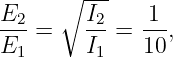
For a plane-like far-field wave,
and similarly I ∝ B2. Hence
and
The sphere area grows as 4πr2, so the same total power is distributed over an area
proportional to r2. Since intensity is quadratic in field amplitude, the amplitudes fall only as
1∕r.
Solution 12: transmitter gain, power density, and received field strength
The equivalent isotropic power in the receiver direction is
The corresponding far-field intensity is
| I | =  | (144)
|
| =  | (145)
|
| = 4.77 × 10⁻⁴ W/m2. | (146) |
Using
we obtain
| Erms | =  | (148)
|
| = 0.424 V/m. | (149) |
Thus
These values assume lossless free-space propagation in the antenna far field and use the specified
directional gain.
Solution 13: why power uses 10 log 10 but field amplitude uses 20 log 10
Because
we have
10 log 10 | = 10 log 10![[( )2]
E2-
E1](https://images.physicslibrary.org/cache/objects/1242/make4ht/ElectromagneticWavesElectromagneticEnergyPoyntingVectorAndIntensityExercisesAndCompleteWorkedSolutions126x.png) | (152)
|
| = 20 log 10 . . | (153) |
If distance doubles, spherical spreading gives
and
Therefore,
| 10 log 10(1∕4) | = −6.02 dB, | (156)
|
| 20 log 10(1∕2) | = −6.02 dB. | (157) |
The factor of 20 for amplitude is not a different physical loss law; it arises because power is
proportional to amplitude squared.
Solution 14: standing waves can store energy without carrying net average power
The Poynting vector is
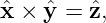
Since x ×y = z,
| S(z,t) | =  ![[2E0 cos(kz)cos(ωt)]](https://images.physicslibrary.org/cache/objects/1242/make4ht/ElectromagneticWavesElectromagneticEnergyPoyntingVectorAndIntensityExercisesAndCompleteWorkedSolutions132x.png) ![[ E ]
2--0sin(kz) sin(ωt )
c](https://images.physicslibrary.org/cache/objects/1242/make4ht/ElectromagneticWavesElectromagneticEnergyPoyntingVectorAndIntensityExercisesAndCompleteWorkedSolutions133x.png) z z | (159)
|
| =  cos(kz) sin(kz) cos(ωt) sin(ωt)z. cos(kz) sin(kz) cos(ωt) sin(ωt)z. | (160) |
Using
we obtain
The average of sin(2ωt) over a full period is zero, so
The electric and magnetic fields still possess nonzero energy density. In a Standing
Wave, energy moves locally back and forth between regions and between electric and
magnetic storage, but there is no net time-averaged transport in either propagation
direction.
Solution 15: electromagnetic energy carried by a finite pulse
The average transported power is
| P | = IA | (164)
|
| = (3.0 × 10⁴)(0.010) | (165)
|
| = 300 W. | (166) |
The pulse energy is
| U | = PΔt | (167)
|
| = (300)(20 × 10−9) | (168)
|
| = 6.0 × 10⁻⁶ J. | (169) |
Thus,
The spatial pulse length is
| L | = cΔt | (171)
|
| = (2.998 × 10⁸)(20 × 10−9) | (172)
|
| = 6.00 m. | (173) |
Its volume is
Therefore the average energy density inside the pulse is
| u | =  | (175)
|
| = 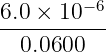 | (176)
|
| = 1.0 × 10⁻⁴ J/m3. | (177) |
Finally,
 | = 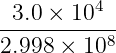 | (178)
|
| = 1.00 × 10⁻⁴ J/m3, | (179) |
which agrees with u = I∕c for the averaged plane-wave quantities.
Solution 16: Julia check of inverse-square and inverse-distance scaling
One direct implementation is:
using Printf

P = 1.0
Z0 = 376.730313668

r = 10 .^ range(0.0, 2.0, length=101)
I = P ./ (4*pi .* r.^2)
E = sqrt.(Z0 .* I)

# Endpoint log-log slopes
slope_I = (log(I[end]) - log(I[1])) / (log(r[end]) - log(r[1]))
slope_E = (log(E[end]) - log(E[1])) / (log(r[end]) - log(r[1]))

@printf("slope of I(r) = %.6f\n", slope_I)
@printf("slope of E(r) = %.6f\n", slope_E)

@printf("I(1 m) = %.6e W/m^2\n", I[1])
@printf("I(100 m) = %.6e W/m^2\n", I[end])
@printf("E(1 m) = %.6e V/m RMS\n", E[1])
@printf("E(100 m) = %.6e V/m RMS\n", E[end])
Because the formulas are exact powers of r, the logarithms are
and
Therefore the expected numerical slopes are
This computational check makes the distinction between power spreading and amplitude spreading
especially clear.
What EM17E1 adds to the series
EM17 established the energy interpretation of the electromagnetic field. EM17E1 makes that
interpretation operational. The worked problems connect stored field energy, local energy transfer,
boundary flux, plane-wave intensity, antenna power density, and geometric spreading through one
conservation framework.
The key chain is
The next article can build naturally from energy flow to electromagnetic momentum, radiation
pressure, or from intensity to antenna reception and effective aperture.
References
[1] David J. Griffiths, Introduction to Electrodynamics, 4th ed., Cambridge University
Press, 2017.
[2] Edward M. Purcell and David J. Morin, Electricity and Magnetism, 3rd ed.,
Cambridge University Press, 2013.
[3] Samuel J. Ling, Jeff Sanny, and William Moebs, University Physics, Volume 2,
OpenStax, 2016, sections on electromagnetic waves, energy, and intensity.
[4] Richard P. Feynman, Robert B. Leighton, and Matthew Sands, The Feynman Lectures
on Physics, Volume II, Addison-Wesley, 1964, chapters on electromagnetic energy and
field flow.
[5] Massachusetts Institute of Technology, 8.02 Physics II: Electricity and Magnetism,
MIT OpenCourseWare, materials on Maxwell’s equations, electromagnetic waves, energy,
and the Poynting vector.

![[parent]](https://images.physicslibrary.org/images/uparrow.png)