Calculus of Variations: Beltrami Problems and Catenary-Type Examples
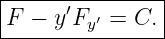
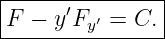
CV06 derived the Beltrami identity for an autonomous first-order functional
namely
The importance of this identity is computational: it replaces the usual second-order
Euler–Lagrange equation by a first-order relation. In favorable cases that relation can be solved
directly for y′ and then integrated by a single quadrature. This companion set develops that skill
through increasingly physical examples, culminating in the catenary and catenoid and ending with
a preview of the brachistochrone [1, 2, 3].
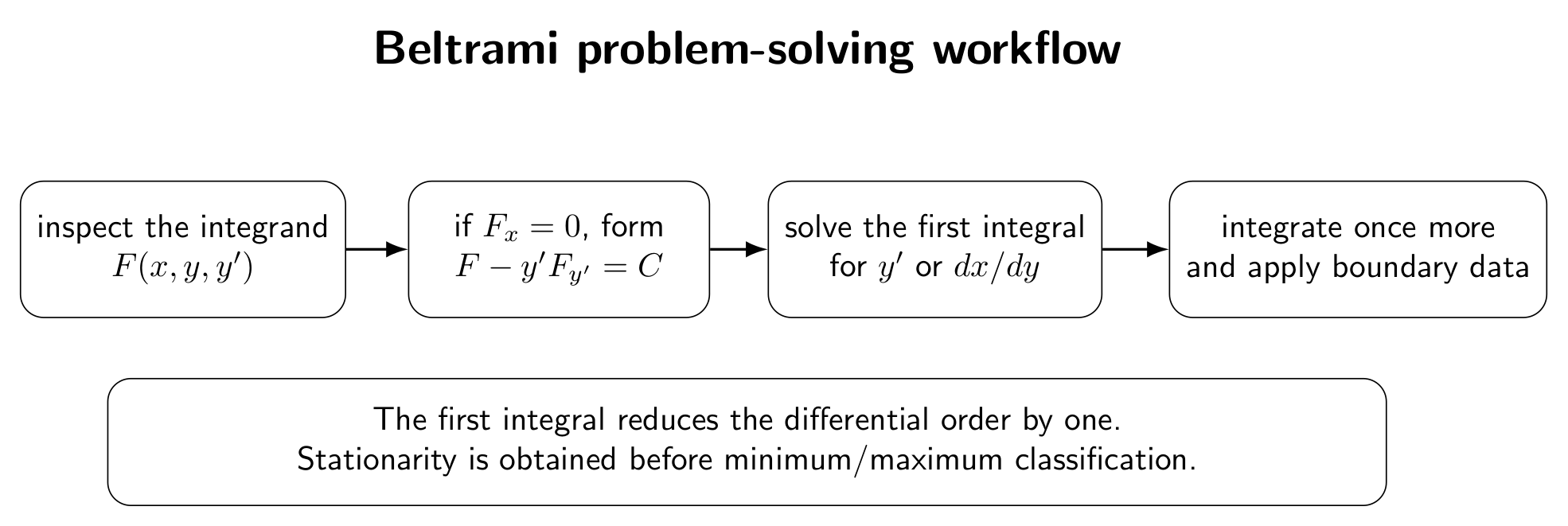
Figure. The practical Beltrami workflow. Autonomy in the independent variable produces
a first integral, which is then solved for the slope and reduced to a quadrature. boundary
data determine the integration constants only after the reduction is complete.
1 How to use this set
Attempt every exercise before reading Part II. For each problem, use the same sequence:
- identify the integrand F and verify that Fx = 0;
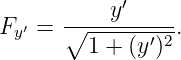
- compute Fy′ carefully;
- form F − y′Fy′ before simplifying;
- set the result equal to a constant;
- solve the first-order relation for y′ or dx∕dy;
- integrate once more, keeping track of branches and constants;
- apply endpoint or symmetry data only after the general stationary family has been
obtained; and
- remember that satisfying Beltrami proves stationarity under the stated hypotheses,
not automatically global minimality.
Part I: Exercises
Exercise 1: recognize when Beltrami applies
For each integrand below, state whether the Beltrami identity can be used immediately. If it can,
compute the corresponding first integral.
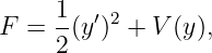
- F =
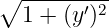 .
.
- F =
 (y′)2 + V (y).
- F = x2(y′)2 + y2.
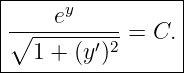
- F = ey
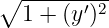 .
.
- F = (1 + x)(y′)2.
For the cases where Beltrami does not apply, identify the explicit dependence that prevents its
direct use.
Exercise 2: a master weighted-length family
Consider
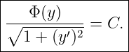
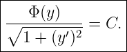
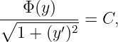
- Use Beltrami to show that every sufficiently smooth stationary curve satisfies
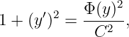
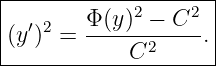
- Solve for (y′)2.
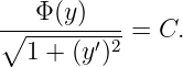
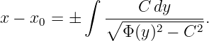
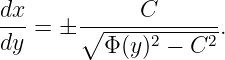
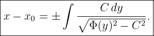
- Derive the quadrature
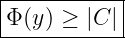
- Explain why the condition Φ(y) ≥|C| appears automatically.
This exercise is the common algebraic core of several later examples.
Exercise 3: shortest path in the plane revisited
For the arc-length functional
use Beltrami, rather than the full Euler–Lagrange equation, to show that every smooth stationary
graph has constant slope and is therefore a straight line. Then impose
and obtain the explicit stationary curve.
Exercise 4: the catenary from an augmented chain functional
A uniform flexible chain in a vertical plane has gravitational potential energy proportional
to
Its total length is fixed. Introducing a constant multiplier λ for that length constraint gives the
augmented integrand
For this exercise, take the augmented functional as given; CV09 will derive the variational
multiplier rule systematically.
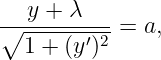
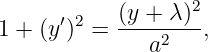
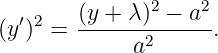
- Apply Beltrami and show that
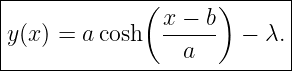
where a > 0 is a constant.
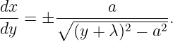
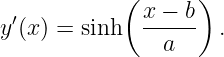
- Solve for y′ and separate variables.
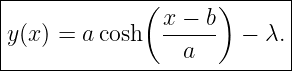
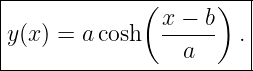
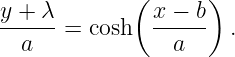
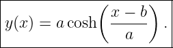
- Integrate to obtain
- Show that the lowest point occurs at x = b and has horizontal tangent.
- Explain which constants are fixed by geometry and which constant is associated with the
length constraint.
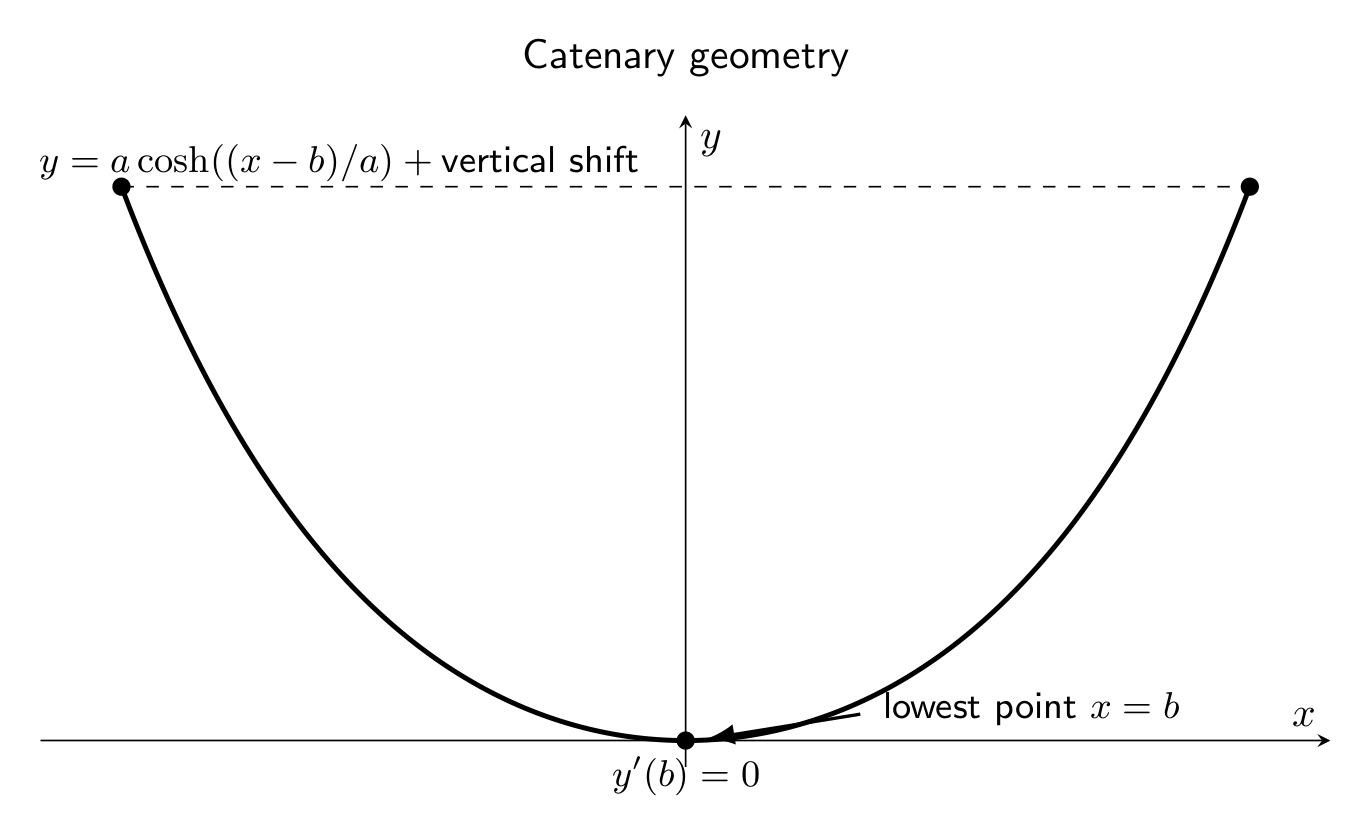
Figure. A catenary-type stationary profile. The parameter b locates the lowest point, a
controls the curvature scale, and an additive vertical shift is absorbed by the multiplier
constant in the augmented formulation.
Exercise 5: why a shallow catenary looks parabolic
For the symmetric catenary
use the Taylor expansion of cosh z to show that, for |x|≪ a,
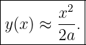
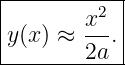
Hence derive the leading parabolic approximation
Estimate the first neglected correction term and explain why a hanging cable with small sag can
appear almost parabolic even though its exact ideal-chain shape is a catenary.
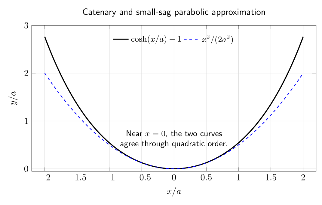
Figure. A symmetric catenary and its small-sag parabolic approximation. The two agree
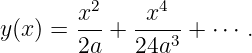
near the lowest point because cosh z = 1 + z2∕2 + O(z4).
Exercise 6: the catenoid from minimum surface area
A surface of revolution is formed by rotating the graph y(x) > 0 about the x-axis. Its area
is
- Ignore the constant factor 2π and apply Beltrami.
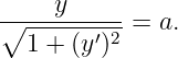
- Show that
- Integrate the first-order equation and obtain
- Explain why the same hyperbolic cosine appears in both the hanging chain and
minimum-surface problems even though the physical functionals are different.
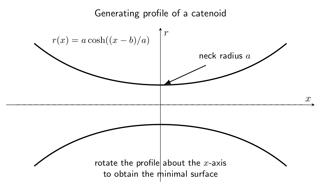
Figure. The generating curve of a catenoid. Rotating the catenary-shaped profile about
the horizontal axis produces the classical minimal surface of revolution.
Exercise 7: autonomous mechanics and the energy integral
Let the independent variable be time t and write qt = dq∕dt. Consider the action
- Apply the Beltrami identity with F = L(q,qt).
- Show that the result can be written
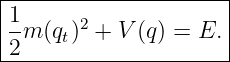
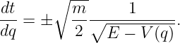
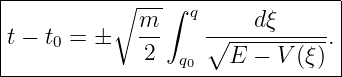
- Solve for dt∕dq and obtain the quadrature
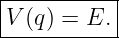
- Explain why turning points satisfy V (q) = E.
Exercise 8: brachistochrone preview by Beltrami
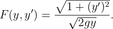
Let y measure vertical distance downward from the starting point. Conservation of mechanical
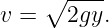
energy gives speed
The travel time along a graph y(x) is therefore
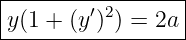
- Apply Beltrami and show that the first integral is equivalent to
for some positive constant a.
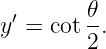
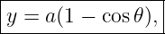
- Introduce the parameter
and show that
- Derive
which is a cycloid.
- Explain why this exercise is only a preview: CV17 will address the historical problem,
endpoint geometry, and full interpretation in detail.
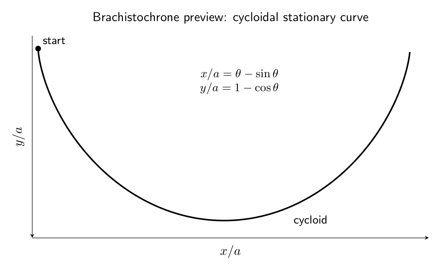
Figure. The Beltrami reduction of the brachistochrone leads naturally to a cycloidal
parameterization. The curve is shown only as a preview of the full CV17 analysis.
Part II: Complete Worked Solutions
Solution 1: recognize when Beltrami applies
Beltrami requires that the integrand have no explicit dependence on the independent variable
x.
(a)
For
we have Fx = 0. Also
Thus
| F − y′Fy′ | = 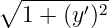 − −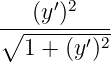 | (29)
|
| = 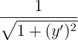 = C. = C. | (30) |
(b)
For
again Fx = 0. Since Fy′ = y′,
(c)
The integrand
contains x explicitly, so Beltrami does not apply directly.
(d)
For
there is no explicit x dependence. Therefore
(e)
The factor (1 + x) is explicit x dependence, so the Beltrami identity cannot be replaced
by a constant. The more general du Bois–Reymond identity from CV06 must be used
instead.
Solution 2: a master weighted-length family
Let
Because Fx = 0, Beltrami gives
First compute
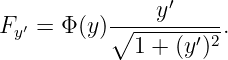
Therefore
| F − y′Fy′ | = Φ(y)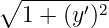 − Φ(y) − Φ(y)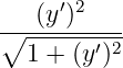 | (39)
|
| = 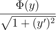 . . | (40) |
Hence
Squaring gives
so
On an interval where a consistent branch is chosen,
Integrating,
For the square root to remain real,
or
because Φ > 0. This restriction is not imposed separately; it is encoded in the first integral
itself.
Solution 3: shortest path in the plane revisited
Here
From Solution 1,
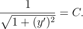
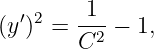
Therefore
which is constant. Choosing one continuous branch,
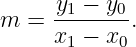
where m is constant. Hence
Apply the two endpoint conditions:
Subtracting,
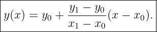
Thus
Beltrami has recovered the same stationary line as the full Euler–Lagrange calculation, but with
one fewer differentiation step.
Solution 4: the catenary from an augmented chain functional
Take
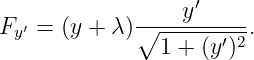
There is no explicit x dependence. Compute
Then
| F − y′Fy′ | = (y + λ)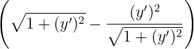 | (58)
|
| = 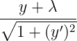 . . | (59) |
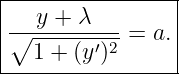
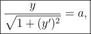
Set the constant equal to a positive parameter a:
Rearrange:
so
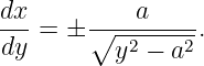
Invert the derivative on a monotone branch:
Let
Then
Because cosh is even, both branches combine into
Therefore
Differentiate:
Thus
and since cosh z ≥ 1, the point x = b is the lowest point of the curve for this sign convention.
The constant b locates the horizontal position of the lowest point. The constant a sets the
curvature scale. The multiplier λ enters as a vertical shift in this augmented form and is ultimately
determined together with a and b by the endpoint geometry and the prescribed total chain length.
The justification for introducing λ as a variational multiplier is the subject of CV09
[1, 2].
Solution 5: why a shallow catenary looks parabolic
Use
With z = x∕a,
| y(x) | = a![[ (x-) ]
cosh a − 1](https://images.physicslibrary.org/cache/objects/1203/make4ht/CalculusOfVariationsBeltramiProblemsAndCatenaryTypeExamples75x.png) | (71)
|
| = a![[ 2 4 ]
x---+ -x---+ ⋅⋅ ⋅
2a2 24a4](https://images.physicslibrary.org/cache/objects/1203/make4ht/CalculusOfVariationsBeltramiProblemsAndCatenaryTypeExamples76x.png) | (72)
|
| =  + +  + +  . . | (73) |
Therefore, when |x|∕a ≪ 1,
The leading neglected term is
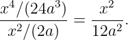
Relative to the quadratic term, its size is approximately
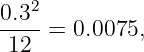
Thus if |x|∕a = 0.3, for example, the first correction is only about
or less than one percent of the quadratic term. This is why shallow catenaries are visually difficult
to distinguish from parabolas over a limited span.
Solution 6: the catenoid from minimum surface area
Ignoring the constant factor 2π, the integrand is
Beltrami gives
Since
we obtain
where a > 0. Rearranging,
Thus
Integrating exactly as in the catenary calculation gives
The repeated hyperbolic cosine is not an accident. Both problems reduce to an integrand of the
general weighted-length form
with a weight linear in y after a vertical shift. The physical meanings are different: the catenary
comes from gravitational potential energy with a length constraint, while the catenoid comes from
surface area. The algebraic structure of the Beltrami first integral is nevertheless the same
[3, 2].
Solution 7: autonomous mechanics and the energy integral
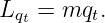
Let
Because L has no explicit time dependence, Beltrami gives
Now
Therefore
| L − qt Lqt | =  m(qt)2 − V (q) − m(q
t)2 m(qt)2 − V (q) − m(q
t)2 | (89)
|
| = −![[ ]
1m (q )2 + V(q)
2 t](https://images.physicslibrary.org/cache/objects/1203/make4ht/CalculusOfVariationsBeltramiProblemsAndCatenaryTypeExamples96x.png) . . | (90) |
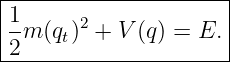
Writing C = −E gives
Solve for qt:
Invert:
Hence
At a turning point, qt = 0. Therefore the energy equation requires
This is the familiar mechanical energy integral, obtained here as a direct Beltrami first integral of
an autonomous action [4, 5].
Solution 8: brachistochrone preview by Beltrami
The integrand is
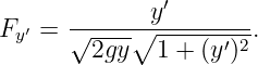
There is no explicit x dependence. Compute
Then
| F − y′Fy′ | =  ![[∘ --------- ′ 2 ]
1 + (y ′)2 − ∘--(y-)----
1 + (y′)2](https://images.physicslibrary.org/cache/objects/1203/make4ht/CalculusOfVariationsBeltramiProblemsAndCatenaryTypeExamples105x.png) | (98)
|
| = 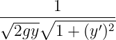 = C. = C. | (99) |
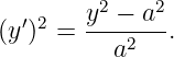
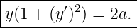
Square and absorb the positive constants into a new parameter a:
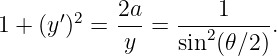
Now set
The first integral gives
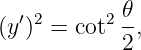
Therefore
and on the descending branch
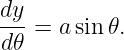
Differentiate the parameterization of y:
Since
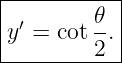
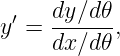
we have
 | =  | (107)
|
| = a sin 𝜃 tan  | (108)
|
| = a(1 − cos 𝜃). | (109) |
Integrating,
Together with
this is the parametric equation of a cycloid. The appearance of the cycloid is one of
the classical achievements of the early calculus of variations. CV17 will return to the
brachistochrone with its historical development and complete variational interpretation
[1, 3].
What these problems should teach
The most important lesson is not that several famous curves can be memorized. It is that one
structural observation,
changes the solution strategy. Rather than expand the full Euler–Lagrange equation into a
second-order ODE, first form
For weighted-length integrands of the form
this immediately becomes
which often exposes the geometry of the problem before any difficult integration begins.
Common mistakes
- Using Beltrami when F contains x explicitly. The constant first integral requires
Fx = 0.
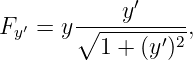
- Computing Fy′ incorrectly. In Φ(y)
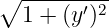 , the factor Φ(y) is held constant
when taking the partial derivative with respect to y′.
, the factor Φ(y) is held constant
when taking the partial derivative with respect to y′.
- Dropping the square-root domain condition. Solving for y′ can introduce a
requirement such as Φ(y)2 ≥ C2.
- Forgetting the branch sign. A first-order relation usually gives y′ = ±f(y). A
complete smooth curve may switch monotone branches at a turning point.
- Treating the multiplier λ in the catenary as arbitrary decoration. It enforces
the fixed-length constraint; CV09 provides the theorem justifying it.
- Calling every hyperbolic-cosine graph a hanging chain. The same analytic
profile also generates a catenoid, but the underlying variational functional is different.
- Assuming a first integral proves a minimum. Beltrami supplies a necessary
stationarity relation. Classification is a separate issue.
Summary
For an autonomous functional
stationarity implies the Beltrami identity
For the common weighted-length family
this reduces to
The same algebraic structure produces a straight line for ordinary planar arc length, a
hyperbolic cosine for the catenary and catenoid, an energy integral in autonomous mechanics,
and the first-order cycloidal relation in the brachistochrone. CV06E2 next emphasizes
the complementary special case of cyclic dependent variables and conserved conjugate
momenta.
References
[1] I. M. Gelfand and S. V. Fomin, Calculus of Variations, Dover Publications, 2000.
[2] Bruce van Brunt, The Calculus of Variations, Springer, 2004.
[3] Robert Weinstock, Calculus of Variations with Applications to Physics and
Engineering, Dover Publications, 1974.
[4] Cornelius Lanczos, The Variational Principles of Mechanics, 4th ed., Dover
Publications, 1986.
[5] Herbert Goldstein, Charles Poole, and John Safko, Classical Mechanics, 3rd ed.,
Addison Wesley, 2002.

![[parent]](https://images.physicslibrary.org/images/uparrow.png)
![∫ b
J[y] = F (y,y′)dx,
a](https://images.physicslibrary.org/cache/objects/1203/make4ht/CalculusOfVariationsBeltramiProblemsAndCatenaryTypeExamples0x.png)
![∫ b ---------
J [y] = Φ (y)∘ 1 + (y′)2dx, Φ(y) > 0.
a](https://images.physicslibrary.org/cache/objects/1203/make4ht/CalculusOfVariationsBeltramiProblemsAndCatenaryTypeExamples5x.png)
![∫ x1∘ ---------
L[y] = 1 + (y ′)2dx,
x0](https://images.physicslibrary.org/cache/objects/1203/make4ht/CalculusOfVariationsBeltramiProblemsAndCatenaryTypeExamples8x.png)




![∫
x1 ∘ ------′2-
A [y] = 2π y 1 + (y ) dx.
x0](https://images.physicslibrary.org/cache/objects/1203/make4ht/CalculusOfVariationsBeltramiProblemsAndCatenaryTypeExamples17x.png)
![∫ t [ ]
1 1- 2
S[q] = t 2 m (qt) − V(q) dt.
0](https://images.physicslibrary.org/cache/objects/1203/make4ht/CalculusOfVariationsBeltramiProblemsAndCatenaryTypeExamples20x.png)

![∫ ∘ ---------
---1 +-(y′)2
T[y] = √2gy-- dx.](https://images.physicslibrary.org/cache/objects/1203/make4ht/CalculusOfVariationsBeltramiProblemsAndCatenaryTypeExamples24x.png)
























![∘ --------------
-2
qt = ± m [E − V (q)].](https://images.physicslibrary.org/cache/objects/1203/make4ht/CalculusOfVariationsBeltramiProblemsAndCatenaryTypeExamples98x.png)





![∫
′
J [y ] = F (y,y) dx,](https://images.physicslibrary.org/cache/objects/1203/make4ht/CalculusOfVariationsBeltramiProblemsAndCatenaryTypeExamples124x.png)