Wave Mechanics: Wave Intensity and Flux
WM18 introduced the energy carried by a one-dimensional wave, and WM19–WM20
developed the instantaneous and average power transported through a fixed point on an
ideal string. The next step is to distinguish total power from power distributed over an
area.
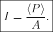
For a wave whose average power ⟨P⟩ is distributed uniformly across an area A, the wave intensity
is
The SI unit of intensity is
Intensity is therefore an areal energy-flux density: it tells us how much energy per unit time crosses
each unit area perpendicular to the direction of transport [3, 4, 1, 2].
This distinction becomes essential when waves spread in two or three dimensions. A
source may emit the same total power while that power is distributed over an ever larger
wavefront. In that situation the total power can remain constant even while the intensity
decreases.
1 Power is not the same as intensity
Power measures the rate of energy transfer:
Its unit is the watt:
Intensity divides that transported power by area:
Thus two waves can carry the same total power but have very different intensities if they occupy
different cross-sectional areas.
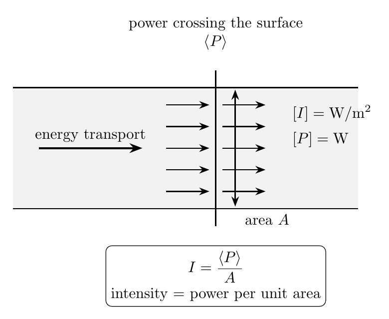
Figure. Intensity is average wave power per unit area measured through a surface
perpendicular to the direction of energy transport.
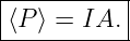
For a uniform intensity over the surface,
This simple relation will appear repeatedly in acoustics, optics, electromagnetic waves, and other
wave systems.
2 Geometric spreading
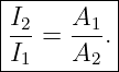
Suppose the same average power passes through two perpendicular surfaces with areas A1 and A2.
If there is no absorption or other loss between the surfaces,
Therefore
If the area increases, the intensity decreases even though the total transported power remains the
same.
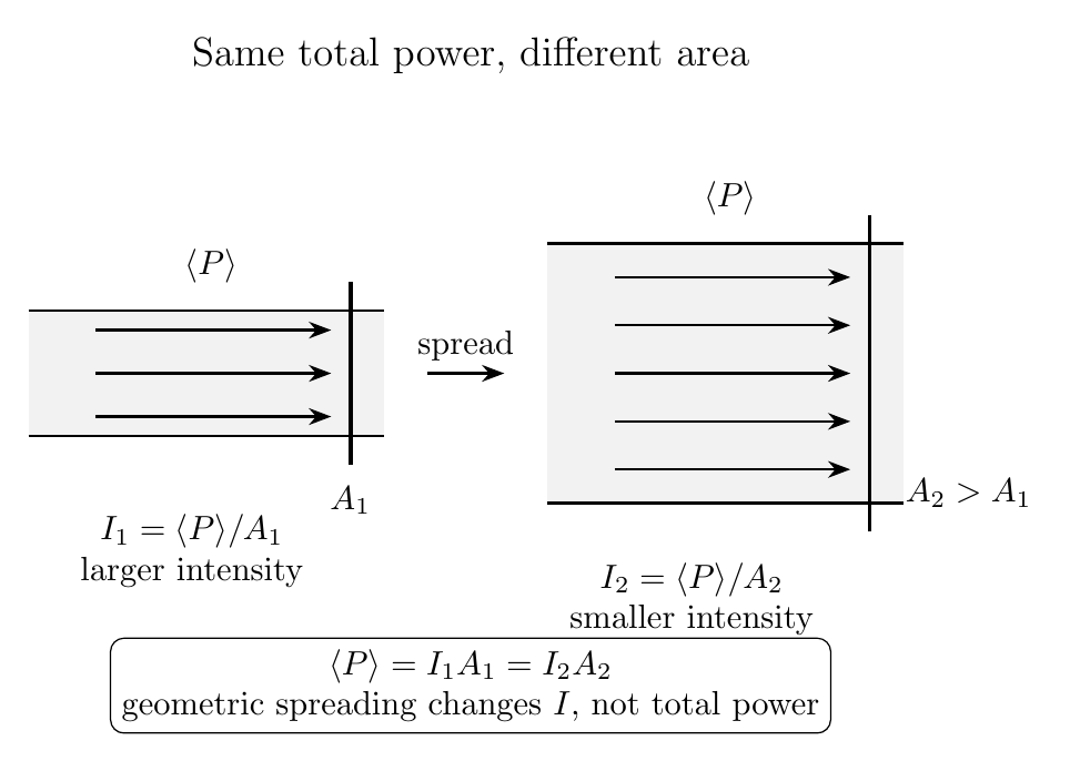
Figure. The same total power distributed over a larger area produces a smaller intensity.
This is geometric spreading, not necessarily dissipative loss.
This distinction is important:
- geometric spreading redistributes the same power over a larger area;
- dissipation or absorption converts some wave energy into other forms, reducing the
power that remains in the wave.
A measured decrease in intensity can result from either effect, so the changing wavefront area must
be considered before concluding that energy has been dissipated.
3 Energy flux as a vector quantity
In more than one spatial dimension, energy transport has a direction as well as a magnitude.
Introduce an energy-flux vector
with units
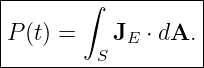
The instantaneous power crossing an oriented surface S is
Here
points normal to the surface.
If the flux is uniform over a flat area and makes an angle α with the surface normal,
then
The largest power crosses when the surface is perpendicular to the direction of propagation, so
α = 0 and
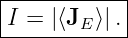
For a steady or periodic wave, the scalar intensity is commonly the magnitude of the time-averaged
energy flux in the propagation direction:
When direction matters, keeping the vector or signed flux is more informative than using only the
positive scalar intensity.
4 Local conservation of wave energy
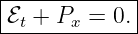
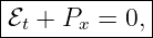
WM19 obtained the one-dimensional conservation law
where ℰ is energy per unit length and P is signed power along the string.
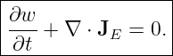
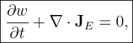
The corresponding three-dimensional local conservation law is
where w is energy per unit volume:
The divergence term measures the net outward energy flux from a small volume. If more energy
flows out than flows in, the energy stored inside must decrease.
This is the same bookkeeping principle used in WM19, now written in a form appropriate to
multidimensional waves [2, 6].
5 Connecting the 1D string to a 3D flux density
Suppose, only for the purpose of connecting the dimensions, that a one-dimensional wave model
represents a uniform wave field across a constant area A. Then
and
Dividing the 1D conservation equation by A gives the corresponding 3D density form.
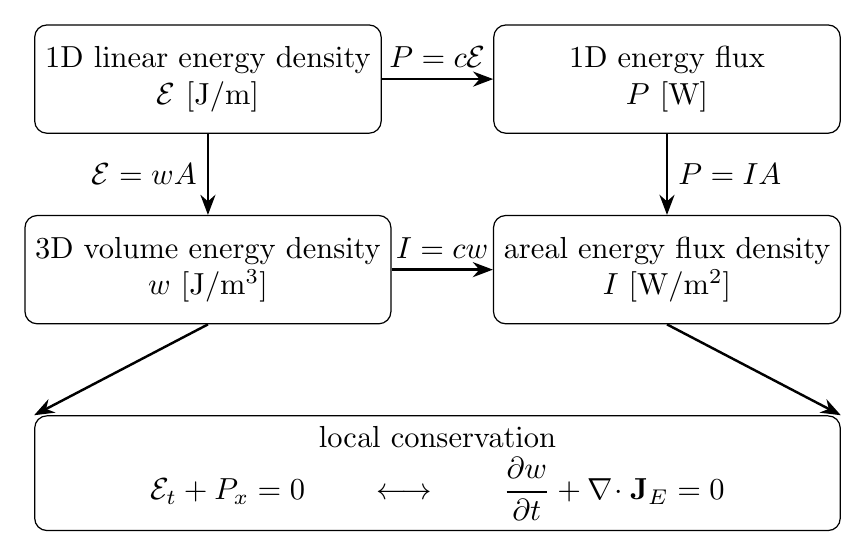
Figure. The one-dimensional quantities ℰ and P correspond to volume energy density w
and areal energy flux density I when a uniform cross-sectional area is introduced.
For the ideal string, P is the natural flux quantity. The string model does not require an areal
intensity because its energy density was defined per unit length rather than per unit volume.
Introducing I = P∕A is therefore a bridge to higher-dimensional wave fields, not a replacement for
the 1D string power.
6 Intensity and energy density for a progressive wave
WM19 showed that for a pure right-moving nondispersive wave on an ideal string,
If
and
then
Canceling the area gives
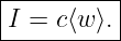
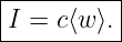
For a periodic wave the corresponding average relation is
This result has a simple interpretation: energy density tells us how much energy occupies a unit
volume, while multiplication by the propagation speed tells us how rapidly that energy sweeps
through a unit area.
The relation I = cw is especially natural for a single progressive nondispersive wave. It should not
be applied blindly to Standing Waves, arbitrary multidirectional fields, or dispersive media without
reconsidering the appropriate energy-transport velocity.
7 Spherical spreading and the inverse-square law
Consider an ideal isotropic point source emitting average power
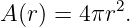
At distance r, the power is distributed uniformly over a spherical surface with area
If no power is lost between the source and the sphere, then
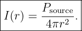
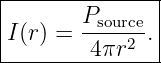
Therefore
This gives the inverse-square law
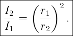
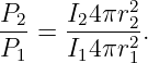
For two radii,
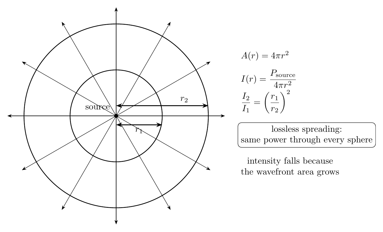
Figure. For an ideal isotropic spherical wave, the same source power crosses every sphere.
Intensity decreases as 1∕r2 because the area grows as 4πr2 [3, 4].
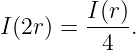
Doubling the distance gives
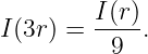
Tripling the distance gives
Again, this decrease does not by itself imply energy loss. It can occur entirely because of geometric
spreading.
8 Different spreading geometries
The dependence of intensity on distance is controlled by the area of the wavefront.
For an ideal plane wave with constant cross-sectional area,
in the absence of loss.
For a cylindrically spreading wave, the wavefront area per fixed axial length grows proportional to
r, so
For a spherical wave,
Thus the familiar inverse-square law is not a universal property of all waves. It is a consequence of
spherical geometry.
9 Intensity and wave amplitude
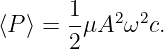
For a linear sinusoidal wave in a fixed medium, average transported power is proportional to the
square of the wave amplitude. WM20 found for the ideal string
The same square-law structure occurs for many other linear wave systems, although the
proportionality constant depends on the medium and on the physical meaning of the
amplitude.
If a spherically spreading linear wave satisfies
and
then its far-field amplitude scales as
This is another way to understand why a wave can become weaker with distance even in a lossless
medium.
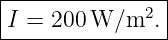
10 Worked Example 1: Convert power to intensity
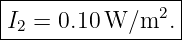
A wave carries an average power
uniformly through an area
Find the intensity.
Solution
Use
Then
| I | =  W∕m2 W∕m2 | (45)
|
| = 200 W∕m2. | (46) |
Therefore
11 Worked Example 2: Spherical spreading
An ideal isotropic source radiates
Find the intensity at r = 3.0 m and at r = 6.0 m.
Solution
At 3.0 m,
| I1 | =  W∕m2 W∕m2 | (49)
|
| ≃ 0.159 W∕m2. | (50) |
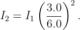
At twice the radius, the inverse-square law gives
Therefore
Thus
and
The total power is unchanged; only the area over which it is distributed has increased.
12 Worked Example 3: Intensity from volume energy density
A progressive wave has average volume energy density
and propagation speed
Find the intensity. Then find the average power through a perpendicular area of 0.40 m2.
Solution
For a progressive nondispersive wave,
Thus
| I | = (340)(0.015) W∕m2 | (58)
|
| = 5.10 W∕m2. | (59) |
The average power is
| ⟨P⟩ | = IA | (60)
|
| = (5.10)(0.40) W | (61)
|
| = 2.04 W. | (62) |
Therefore
13 Worked Example 4: Same power through a larger area
A wave has intensity
through a uniform area
The same total power later occupies an area
Find the new intensity.
Solution
First compute the conserved power:
Then
Therefore
14 Worked Example 5: Bridge from string power to an areal intensity
A sinusoidal wave on an ideal string has
First find the average string power. Then, purely as a dimensional bridge to a uniform
three-dimensional field, suppose that power is distributed over an effective area
Find the corresponding intensity.
Solution
Use the WM20 result
The angular frequency is
With
we obtain
| ⟨P⟩ | =  (0.012)(0.0020)2(80π)2(100) (0.012)(0.0020)2(80π)2(100) | (76)
|
| ≃ 0.152 W. | (77) |
If this power is assigned to the stated effective area,
| I | = 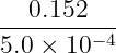 W∕m2 W∕m2 | (78)
|
| ≃ 303 W∕m2. | (79) |
Thus
The string calculation itself needs only ⟨P⟩. The areal intensity appears only after an effective area
is introduced.
15 Worked Example 6: Separate geometric spreading from true loss
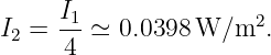
At radius r1 = 2.0 m from a source, an intensity I1 is measured. At radius r2 = 5.0 m, the
measured intensity is
If the wave were lossless and spherically spreading, what ratio would be expected? What fraction
of the power crossing the first sphere remains in the wave at the second sphere?
Solution
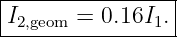
Pure spherical spreading predicts
 | =  2 2 | (82)
|
| =  2 2 | (83)
|
| = 0.16. | (84) |
Thus geometric spreading alone would give
The actual powers through the two spherical surfaces satisfy
Therefore
 | = 0.10 2 2 | (87)
|
| = 0.625. | (88) |
So
of the wave power crossing the inner sphere remains at the outer sphere. The remaining
has been removed from the propagating wave by effects beyond ideal geometric spreading.
16 Common mistakes
- Mistake: treating power and intensity as the same quantity. Power is measured in
watts; intensity is power per unit area.
- Mistake: assuming any decrease in intensity means energy has been dissipated.
Intensity can decrease simply because the wave spreads over a larger area.
- Mistake: applying the spherical inverse-square law to every wave geometry. Plane,
cylindrical, and spherical spreading have different area laws.
- Mistake: forgetting that flux has a direction. The dot product JE ⋅dA determines the
signed power crossing an oriented surface.
- Mistake: applying I = cw to arbitrary standing, dispersive, or multidirectional waves
without checking the transport physics.
- Mistake: assigning a unique areal intensity to the ideal 1D string without first defining
an area. The intrinsic 1D transport quantity is the power P.
17 What WM21 adds to the wave-mechanics picture
The sequence of transport quantities is now
For the one-dimensional string,
For a multidimensional wave field,
For a progressive nondispersive wave,
And for an ideal isotropic spherical source,
These ideas provide the transport language needed later for acoustic intensity, electromagnetic
energy flux, RF propagation, and higher-dimensional wave equations.
References
References
[1] A. P. French, Vibrations and Waves, M.I.T. Introductory Physics Series, W. W.
Norton & Company, 1971.
[2] Frank S. Crawford, Jr., Waves, Berkeley Physics Course, Volume 3, McGraw-Hill,
1968.
[3] William Moebs, Samuel J. Ling, and Jeff Sanny, University Physics, Volume 1,
OpenStax, 2016, Section 16.4, “Energy and Power of a Wave.”
[4] William Moebs, Samuel J. Ling, and Jeff Sanny, University Physics, Volume 1,
OpenStax, 2016, Section 17.3, “Sound Intensity.”
[5] Massachusetts Institute of Technology, 8.03SC Physics III: Vibrations and Waves,
MIT OpenCourseWare, Fall 2016.
[6] Massachusetts Institute of Technology, 2.24 / 13.022 Ocean Wave Interaction with
Ships and Offshore Energy Systems, Lecture 4, “Wave Energy Density and Flux,” MIT
OpenCourseWare, Spring 2002.

![|------------|
[I] = W ∕m2. |
--------------](https://images.physicslibrary.org/cache/objects/1189/make4ht/WaveMechanicsWaveIntensityAndFlux1x.png)

![[P] = W = J ∕s.](https://images.physicslibrary.org/cache/objects/1189/make4ht/WaveMechanicsWaveIntensityAndFlux3x.png)



![[JE ] = W ∕m2.](https://images.physicslibrary.org/cache/objects/1189/make4ht/WaveMechanicsWaveIntensityAndFlux9x.png)



![3
[w ] = J∕m .](https://images.physicslibrary.org/cache/objects/1189/make4ht/WaveMechanicsWaveIntensityAndFlux17x.png)