Wave Mechanics: Initial Conditions and the d'Alembert Solution

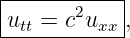
Wave Mechanics: Initial Conditions and the d’Alembert Solution

WM16 established the structural form of a sufficiently smooth solution of the one-dimensional constant-speed wave equation,

|-----------| -utt =-c2uxx-,

(1)

namely

|-------------------------------| |u(x,t) = F (x − ct) + G (x + ct). --------------------------------

(2)

The two arbitrary functions represent independent right- and left-moving components. The remaining question is physical as well as mathematical:

|------------------------------------------------------------------------| -How--do-the-initial-displacement--and-initial-velocity-determine-F--and-G?--|

(3)

The answer is the classical d’Alembert formula for the initial-value problem on the whole line. If

u(x,0) = f(x )

(4)

and

ut(x,0) = g(x ),

(5)

then, under the usual smoothness assumptions,

|----------------------------------------------------| | 1 1 ∫ x+ct | |u(x,t) = --[f (x − ct) + f(x + ct)] + --- g (s) ds.| ----------2--------------------------2c-x−-ct----------

(6)

This formula solves the initial-value problem explicitly and makes finite propagation speed visible in the mathematics [4, 3, 6].

1 Why two initial conditions are needed

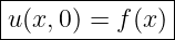
The wave equation contains a second derivative with respect to time. Just as a second-order Ordinary Differential Equation generally requires an initial position and an initial velocity, the wave equation requires two initial functions:

|--------------| |u(x,0) = f(x )| ----------------

(7)

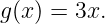
and

|---------------| ut(x,0) = g(x ). | -----------------

(8)

The function f(x) describes the initial shape of the string or wave field. The function g(x) describes the initial velocity of every material point.

The logical structure is summarized below.

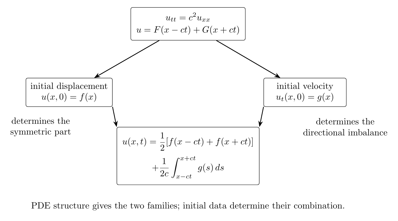
Figure. The wave equation supplies the two traveling families. Initial displacement and initial velocity determine how those families are combined.

2 Apply the initial displacement

Begin with the WM16 form

u(x,t) = F (x − ct) + G (x + ct).

(9)

At t = 0,

u (x,0) = F (x ) + G (x).

(10)

The initial displacement condition therefore gives

|--------------------| F-(x)-+-G-(x) =-f(x).-

(11)

This is one relation between the two unknown functions.

3 Apply the initial velocity

Differentiate the general solution with respect to time:

ut(x,t) = − cF ′(x − ct) + cG ′(x + ct).

(12)

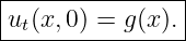
At t = 0,

ut(x,0) = − cF′(x) + cG′(x).

(13)

The initial velocity condition therefore gives

|----′--------′-----------| −-cF-(x)-+-cG-(x)-=-g(x-).--

(14)

Divide by c:

g(x ) − F′(x) + G ′(x) = -----. c

(15)

Meanwhile, differentiating

F (x ) + G (x) = f(x )

(16)

with respect to x gives

F′(x) + G′(x) = f′(x).

(17)

We now have two algebraic equations for the two unknown derivative functions F′ and G′.

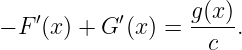
4 Solve for the two traveling components

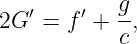
Add the two equations:

F′ + G′	= f′,	(18)
− F′ + G′	= .	(19)

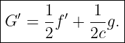
This gives

2G ′ = f ′ + g-, c

(20)

|----------------| | ′ 1- ′ -1- | |G = 2 f + 2c g.| ------------------

(21)

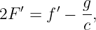
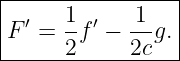
Subtracting instead gives

′ ′ g 2F = f − --, c

(22)

|----------------| | ′ 1- ′ -1- | |F = 2 f − 2c g.| ------------------

(23)

Integrating with respect to the argument gives, for a convenient fixed reference point x_∗,

∫ x F (x) = 1f (x) − 1-- g(s)ds + CF 2 2c x∗

(24)

and

1 1 ∫ x G(x ) = -f(x) + --- g(s)ds + CG. 2 2c x∗

(25)

The displacement condition requires the constants to satisfy

CF + CG = 0.

(26)

Only the sum F + G matters physically, so the arbitrary constant split cancels from the final solution.

5 Derive the d’Alembert formula

Substitute x − ct into F and x + ct into G:

u(x,t)	= f(x − ct) + f(x + ct)	(27)
	−∫ _{x_∗}^x−ctg(s) ds + ∫ _{x_∗}^x+ctg(s) ds.	(28)

Using

∫ ∫ ∫ x+ct x−ct x+ct g (s )ds − g(s)ds = g(s)ds, x∗ x∗ x−ct

(29)

we obtain

|----------------------------------------------------| | 1 1 ∫ x+ct | |u(x,t) = --[f (x − ct) + f(x + ct)] + --- g (s) ds.| ----------2--------------------------2c-x−-ct----------

(30)

This is the d’Alembert solution of the one-dimensional wave equation initial-value problem on the whole line [4, 6].

6 Interpret the displacement term

First suppose the initial velocity is zero:

g(x) = 0.

(31)

Then

|----------------------------------| | 1- 1- | |u(x,t) = 2 f(x − ct) + 2 f(x + ct). -----------------------------------

(32)

The initial shape splits into two copies. One moves right, one moves left, and each has half the original amplitude.

At t = 0 the copies overlap exactly:

1f(x) + 1-f(x) = f(x). 2 2

(33)

The splitting is illustrated below.

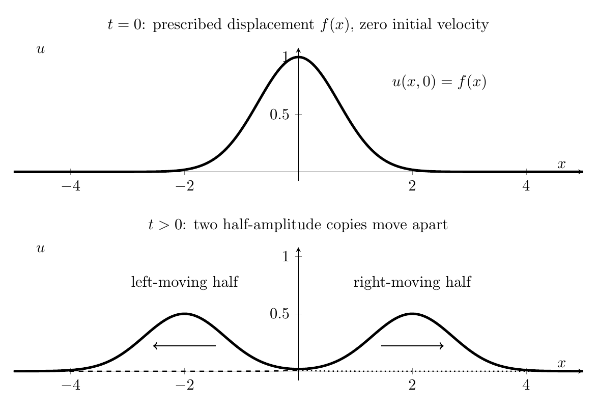
Figure. With zero initial velocity, the initial displacement profile separates into equal right- and left-moving half-amplitude copies.

This result is one of the clearest physical interpretations of the d’Alembert formula.

7 Interpret the velocity term

Now suppose the initial displacement is zero:

f(x ) = 0.

(34)

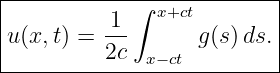
Then

|------------∫-------------| | -1- x+ct | |u(x,t) = 2c g(s)ds. | --------------x−ct---------

(35)

The displacement at (x,t) depends on the accumulated initial velocity over the interval

[x − ct, x + ct].

(36)

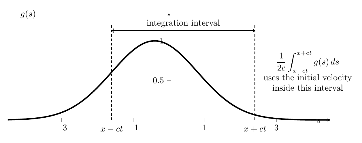
Figure. The initial-velocity contribution is determined by the integral of g(s) over the characteristic interval from x − ct to x + ct.

The width of that interval is

2ct.

(37)

As time increases, information from a larger portion of the initial line can influence the observation point.

8 Domain of dependence and finite propagation speed

For a point (x₀,t₀), the d’Alembert formula uses initial data only between

x0 − ct0

(38)

and

x0 + ct0.

(39)

These endpoints are reached by the two backward characteristic lines.

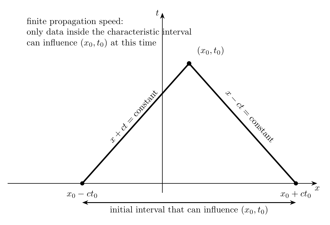
Figure. The value at (x₀,t₀) depends only on initial data in the interval [x₀ − ct₀,x₀ + ct₀]. This is the domain of dependence for the one-dimensional constant-speed wave equation.

Therefore a disturbance in the initial data cannot influence arbitrarily distant points instantaneously. Information propagates at the finite speed c.

This causal structure is one of the most important qualitative consequences of the wave equation [4].

9 Pure one-way motion requires compatible initial data

The d’Alembert formula also reveals the initial-data condition for a wave to travel in only one direction.

For a pure right-moving wave,

u(x,t) = F (x − ct).

(40)

At t = 0,

f(x) = F (x)

(41)

and

g(x) = − cF′(x).

(42)

Therefore

|------------------------------------------------------| g (x) = − cf ′(x) produces a pure right-moving wave. | --------------------------------------------------------

(43)

Similarly,

|-----------------------------------------------------| | ′ | g(x-) =-+cf-(x)-----produces-a-pure-left-moving--wave.--

(44)

This explains why an arbitrary initial shape by itself does not usually travel in only one direction. The initial velocity must be chosen consistently with the desired direction.

10 Checking the initial conditions directly

A useful consistency check is to set t = 0 in the d’Alembert formula:

u(x, 0)	= [f(x) + f(x)] + ∫ _x^xg(s) ds	(45)
	= f(x).	(46)

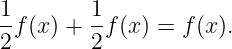
Thus the displacement condition is satisfied.

To check the velocity, differentiate the formula with respect to time. The displacement part gives

c ′ c ′ − 2f (x − ct) + 2f (x + ct).

(47)

For the integral term, the Leibniz rule gives

	=	(48)
	= [g(x + ct) + g(x − ct)].	(49)

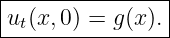
At t = 0, the two f′ terms cancel and the velocity term becomes

1- 2[g(x) + g(x)] = g(x).

(50)

Therefore

|---------------| ut(x,0) = g(x ). | -----------------

(51)

11 The role of boundaries

The formula derived here is most naturally stated for the initial-value problem on the entire real line.

On a finite interval, boundary conditions also matter. Reflections from fixed or free boundaries can be incorporated through reflected extensions, mode expansions, or other boundary-value methods. The PhysicsLibrary treatment of boundary conditions in WM12 explains why endpoint constraints modify which solutions are physically allowed.

Thus

|--------------------------------------------------------------------------------------| |d’Alembert formula on the whole line ⁄= complete finite-string boundary -value solution. | ---------------------------------------------------------------------------------------

(52)

12 Regularity assumptions

The derivation above assumes enough differentiability for the chain rule, mixed derivatives, and the classical wave equation to be meaningful. A common sufficient setting is to take f twice continuously differentiable and g continuously differentiable.

Less regular initial data can also be treated using weaker notions of solution, but that belongs to a more advanced PDE treatment [4].

13 Worked example 1: released Gaussian displacement

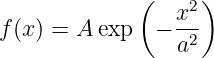
Suppose

( 2) f(x ) = A exp − x-- a2

(53)

and

g(x) = 0.

(54)

The d’Alembert formula immediately gives

u(x,t)	= exp	(55)
	+ exp .	(56)

Therefore the initial Gaussian separates into two Gaussian pulses of amplitude A∕2 traveling in opposite directions at speed c:

|--------------------------------------| |u(x,t) = A-e−(x−ct)2∕a2 + A-e− (x+ct)2∕a2. ----------2---------------2------------|

(57)

At t = 0, the two halves add to recover the original amplitude A.

14 Worked example 2: zero displacement but sinusoidal initial velocity

Suppose

f (x) = 0

(58)

and

g(x) = V0 cos(kx ).

(59)

Then

V0∫ x+ct u (x, t) = --- cos(ks)ds. 2c x−ct

(60)

Integrate:

u(x,t)

(61)

Using

sin(α + β) − sin(α − β ) = 2cos αsin β,

(62)

we obtain

|----------------------------| | V0 | |u(x,t) = ck-cos(kx)sin(kct).| ------------------------------

(63)

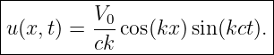
Since

ω = ck,

(64)

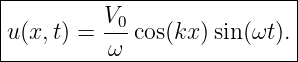
this is a standing-wave form:

|----------------------------| | V0- | |u(x,t) = ω cos(kx )sin (ωt ).| -----------------------------

(65)

Different initial data can therefore generate a standing pattern even though the underlying solution is still built from right- and left-moving components.

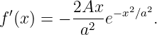
15 Worked example 3: choose data for a pure right-moving pulse

Suppose the desired initial shape is

−x2∕a2 f (x) = Ae .

(66)

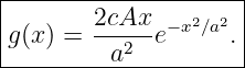
To make it move purely to the right, choose

g(x) = − cf′(x).

(67)

Differentiate:

′ 2Ax--−x2∕a2 f (x) = − a2 e .

(68)

Therefore

|--------------------| | 2cAx--− x2∕a2 | |g(x) = a2 e .| ----------------------

(69)

With this compatible initial velocity, the left-moving component vanishes and

|---------------[----------2]--| |u(x,t) = A exp − (x-−-ct)- .| | a2 | -------------------------------

(70)

The entire initial pulse moves right without splitting.

16 Worked example 4: evaluate the formula numerically

Let

c = 2.0 m/s,

(71)

with initial data

f(x) = x2

(72)

and

g(x) = 3x.

(73)

Find u(1.0 m, 0.25 s).

First compute the characteristic endpoints:

x − ct	= 1.0 − (2.0)(0.25) = 0.50 m,	(74)
x + ct	= 1.0 + (2.0)(0.25) = 1.50 m.	(75)

The displacement contribution is

[f(0.50) + f(1.50)]	= [0.50² + 1.50²]	(76)
	= [0.25 + 2.25]	(77)
	= 1.25.	(78)

The velocity contribution is

∫ _0.50^1.503sds	= _0.50^1.50	(79)
	=	(80)
	= 0.75.	(81)

Therefore

|------------------| |u(1.0,0.25 ) = 2.00 | --------------------

(82)

in the displacement units implied by the chosen initial data.

17 Worked example 5: choose data for a pure left-moving wave

Suppose

f(x) = A cos(kx ).

(83)

To obtain only a left-moving wave, choose

′ g(x) = +cf (x).

(84)

Since

′ f (x) = − Ak sin(kx),

(85)

we require

|---------------------| g(x) = − cAk sin(kx ). | -----------------------

(86)

The resulting solution is

|------------------------| u(x, t) = A cos[k(x + ct)], --------------------------

(87)

or, using ω = ck,

|------------------------| |u(x,t) = A cos(kx + ωt).| --------------------------

(88)

The initial velocity therefore determines which of the two characteristic families survives.

18 Worked example 6: connect d’Alembert’s solution to string mechanics

A string has

T = 144 N

(89)

and

μ = 0.016 kg/m.

(90)

Its wave speed is

c	=	(91)
	=	(92)
	=	(93)
	≈ 94.9 m/s .	(94)

Suppose the initial displacement is

f (x) = 0.010cos(4x )m

(95)

and the initial velocity is zero.

Then

u(x,t)	= 0.005 cos[4(x − ct)]	(96)
	+ 0.005 cos[4(x + ct)].	(97)

Using the cosine sum identity,

u (x,t) = 0.010 cos(4x) cos(4ct).

(98)

The angular frequency is

ω	= ck	(99)
	= (94.9)(4)	(100)
	≈ 380 rad/s .	(101)

Thus

|----------------------------------| -u(x,t) ≈-0.010cos(4x-)cos(380t)m.--

(102)

The same result can be viewed either as two counter-propagating traveling waves or as a standing-wave pattern generated by the specified initial data.

19 Common mistakes

Mistake: using only the initial displacement. A second-order-in-time wave equation also requires the initial velocity.
Mistake: forgetting the factor 1∕2 multiplying the two displaced copies of f.
Mistake: reversing the limits of the velocity integral. The correct interval is from x−ct to x + ct.
Mistake: forgetting the factor 1∕(2c) in front of the velocity integral.
Mistake: assuming zero initial velocity produces one traveling copy of f. It produces equal left- and right-moving half-amplitude copies.
Mistake: using the whole-line formula without considering finite-domain boundary conditions.
Mistake: assuming arbitrary f and g produce a pure one-way wave. Pure right- or left-moving motion requires the compatibility conditions g = ∓cf′.

20 What WM17 establishes

The structural solution from WM16,

u(x,t) = F (x − ct) + G (x + ct),

(103)

becomes a complete initial-value solution once the functions

f(x) = u(x, 0)

(104)

and

g (x) = ut(x, 0)

(105)

are specified:

|----------------------------------------------------| | 1 1 ∫ x+ct | |u(x,t) = --[f(x − ct) + f(x + ct)] +--- g(s) ds.| ----------2-------------------------2c--x−ct---------

(106)

The formula exposes three major physical ideas at once:

waves propagate along two characteristic directions,
information travels at finite speed c, and
both initial displacement and initial velocity are required to determine the subsequent motion.

This completes the basic initial-value solution of the one-dimensional ideal wave equation and prepares the way for later treatments of energy transport, interfaces, modal expansions, Fourier methods, and dispersive wave systems.

References

[1] A. P. French, Vibrations and Waves, M.I.T. Introductory Physics Series, W. W. Norton & Company, 1971.

[2] Frank S. Crawford, Jr., Waves, Berkeley Physics Course, Volume 3, McGraw-Hill, 1968.

[3] Richard P. Feynman, Robert B. Leighton, and Matthew Sands, The Feynman Lectures on Physics, Volume I, Chapter 47, “Sound. The Wave Equation.”

[4] Walter A. Strauss, Partial Differential Equations: An Introduction, Second Edition, John Wiley & Sons, 2008.

[5] Massachusetts Institute of Technology, 8.03SC Physics III: Vibrations and Waves, Lecture 10, “Traveling Waves,” MIT OpenCourseWare.

[6] Gilbert Strang and Cleve Moler, Learn Differential Equations: Up Close, “Wave Equation,” MIT OpenCourseWare, 2015.

"Wave Mechanics: Initial Conditions and the d'Alembert Solution" is owned by bloftin.
(view preamble)