
|
|
|
|||||||
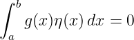
for every admissible test function carries much more information than the same equality for one or finitely many chosen functions.
1 Exercises
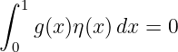
Exercise 1: Hypothesis auditFor each statement below, determine the strongest conclusion that follows and state which version of the Fundamental Lemma is being used.
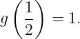
Exercise 2: One test function is not enoughLet
Find a nonzero linear function
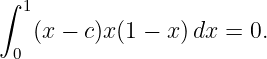
such that
Explain why this does not contradict the Fundamental Lemma.
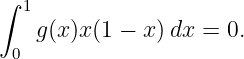
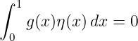
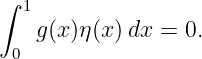
Exercise 3: A weighted-square proofSuppose g ∈ C1([0, 1]) and
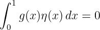
for every η ∈ C1([0, 1]) satisfying η(0) = η(1) = 0. Without invoking the Fundamental Lemma by name, choose a test function depending on g and prove directly that g ≡ 0.
Exercise 4: Recover a differential equation and solve itSuppose y ∈ C2([0, 1]) satisfies
for every η ∈ Cc∞(0, 1), together with
Use the Fundamental Lemma to determine y(x).
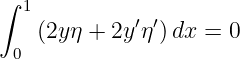
Exercise 5: First variation to boundary-value problemLet y ∈ C2([0, 1]) satisfy the fixed-endpoint stationarity identity
for every η ∈ C1([0, 1]) with η(0) = η(1) = 0. If
derive and solve the differential equation for y.
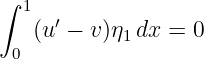
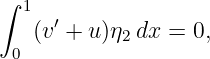
Exercise 6: Vector-valued Fundamental LemmaLet u,v ∈ C1([0, 1]) and suppose
for every pair (η1,η2) of smooth compactly supported test functions.
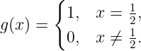
Exercise 7: Pointwise versus almost-everywhere equalityDefine
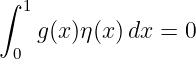
Show that
for every smooth compactly supported test function η. Why is the conclusion g = 0 almost everywhere correct while the conclusion g = 0 at every point is false?
Exercise 8: Stationarity is not classificationConsider
on the fixed-endpoint class y(0) = y(1) = 0.
2 Solutions
Solution 1: Hypothesis audit(a) The classical Fundamental Lemma applies directly. Since g is continuous and the integral vanishes for every smooth compactly supported test function,
for every x ∈ (0, 1), and continuity extends the conclusion to the endpoints. Thus
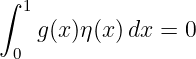
(b) No such conclusion follows. This is one scalar orthogonality condition on an infinite-dimensional set of possible g. A nonzero function can easily have zero weighted integral against a single chosen test function. Exercise 2 constructs one explicitly. (c) The fixed-endpoint corollary applies. Every function in Cc∞(0, 1) is also a C1 function that vanishes at both endpoints, so the hypothesis includes the test class required by the Fundamental Lemma. Therefore
(d) The weak Fundamental Lemma applies. The correct conclusion is
for almost every x ∈ (0, 1). Without additional regularity such as continuity, pointwise equality everywhere cannot be inferred.
Solution 2: One test function is not enoughWe require
Separate the two terms:
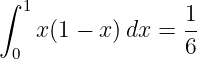
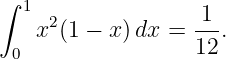
The required integrals are
and
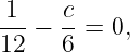
Therefore
so
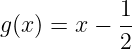
Thus
is nonzero yet satisfies the given integral identity.
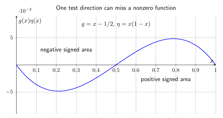
Figure. The product gη is negative on the left half of the interval and positive on the right half. Its signed areas cancel. A single vanishing integral is therefore an orthogonality statement, not a pointwise conclusion. There is no contradiction with the Fundamental Lemma because the lemma assumes that the integral vanishes for every test function in a sufficiently rich class, not for one chosen η.
Solution 3: A weighted-square proofChoose
Because g ∈ C1([0, 1]), this η belongs to C1([0, 1]), and
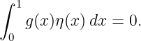
It is therefore an admissible test function. Substitution gives
For 0 < x < 1,
and g(x)2 ≥ 0. Hence the integrand is nonnegative. A continuous nonnegative function with zero integral must vanish identically, so
for every x ∈ [0, 1]. On the open interval this implies
Continuity then gives g(0) = g(1) = 0. Therefore
This proof is efficient, but it relies on the test class being broad enough to allow a test function constructed from g itself.
Solution 4: Recover a differential equation and solve itDefine
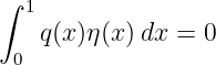
Since y ∈ C2, the function q is continuous. The hypothesis says
for every smooth compactly supported η. The Fundamental Lemma therefore gives
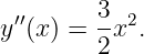
or
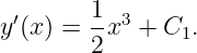
Integrating once,
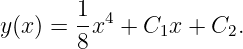
Integrating again,
The condition y(0) = 0 gives C2 = 0. The condition y(1) = 1 gives
hence
Therefore
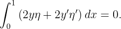
Solution 5: First variation to boundary-value problemBegin with
Integrate the second term by parts:
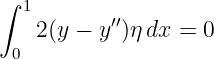
Since η(0) = η(1) = 0, the boundary term vanishes. Thus
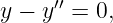
for every fixed-endpoint test function. The Fundamental Lemma gives
or
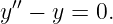
The general solution is
From y(0) = 0,
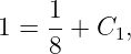
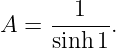
From y(1) = 1,
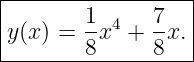
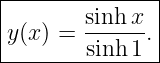
Hence
This exercise exhibits the complete chain that CV03 supports:
Solution 6: Vector-valued Fundamental LemmaBecause the test components are independently arbitrary, choose first
Then
for every scalar test function η1. Hence
Now choose
Then
so
Thus the coupled system is
Figure. A vector test function can be chosen with only one component active. The vector integral identity therefore separates into scalar identities, to which the scalar Fundamental Lemma is applied componentwise. Differentiate u′ = v to obtain
so
Hence
Since v = u′,
The initial data u(0) = 1 and v(0) = 0 give
Therefore
Solution 7: Pointwise versus almost-everywhere equalityThe function g differs from zero at only the single point x = 1∕2. Changing an integrand at a set of measure zero does not change its integral. Therefore for every test function η,
Nevertheless,
Thus pointwise equality everywhere is false. However, the set on which g is nonzero has measure zero, so
This is exactly why the weak Fundamental Lemma concludes almost-everywhere equality for locally integrable functions. Continuity is what upgrades that conclusion to pointwise equality in the classical theorem.
Solution 8: Stationarity is not classificationFor
the first variation is
At y∗ = 0,
so
for every admissible η. Thus y∗ = 0 is stationary. For every admissible y,
At y = 0,
Therefore
The Fundamental Lemma is used when converting a stationary integral identity into a pointwise differential equation. It does not classify a stationary function as a minimum or maximum. Classification here comes from the sign of the functional itself.
3 SummaryThe exercises reinforce four distinct lessons:
"Calculus of Variations Examples: Fundamental Lemma Problems" is owned by bloftin.
This object's parent. Cross-references: system, CV03, boundary, differential equation, function, identities, vector, scalar, theorem There is 1 reference to this object. This is version 1 of Calculus of Variations Examples: Fundamental Lemma Problems, born on 2026-09-10. Object id is 1146, canonical name is CalculusOfVariationsExamplesFundamentalLemmaProblems. Accessed 279 times total. Classification:
|
|
|
|
Pending Errata and AddendaNone.
|
DiscussionNo messages.
|
Interact |
![[parent]](https://images.physicslibrary.org/images/uparrow.png)





![∫ 1
[(u′ − v)η1 + (v′ + u)η2]dx = 0
0](https://images.physicslibrary.org/cache/objects/1146/make4ht/CalculusOfVariationsExamplesFundamentalLemmaProblems13x.png)

![∫
1 ′ 2
J [y] = − y(x ) dx
0](https://images.physicslibrary.org/cache/objects/1146/make4ht/CalculusOfVariationsExamplesFundamentalLemmaProblems17x.png)

![g ≡ 0 on [0,1].](https://images.physicslibrary.org/cache/objects/1146/make4ht/CalculusOfVariationsExamplesFundamentalLemmaProblems19x.png)














![∫ 1 ∫ 1
2y′η′dx = [2y′η]10 − 2y′′η dx.
0 0](https://images.physicslibrary.org/cache/objects/1146/make4ht/CalculusOfVariationsExamplesFundamentalLemmaProblems46x.png)
















![∫ 1 ′2
J [y ] = − y dx,
0](https://images.physicslibrary.org/cache/objects/1146/make4ht/CalculusOfVariationsExamplesFundamentalLemmaProblems71x.png)
![∫ 1
δJ[y;η] = − 2 y′η ′dx.
0](https://images.physicslibrary.org/cache/objects/1146/make4ht/CalculusOfVariationsExamplesFundamentalLemmaProblems72x.png)

![δJ [0;η] = 0](https://images.physicslibrary.org/cache/objects/1146/make4ht/CalculusOfVariationsExamplesFundamentalLemmaProblems74x.png)
![∫
1 ′2
J [y] = − y dx ≤ 0.
0](https://images.physicslibrary.org/cache/objects/1146/make4ht/CalculusOfVariationsExamplesFundamentalLemmaProblems75x.png)
![J [0 ] = 0.](https://images.physicslibrary.org/cache/objects/1146/make4ht/CalculusOfVariationsExamplesFundamentalLemmaProblems76x.png)
