1 The Electric Field of a Line of Charge

Calculating the electric field due to a non-moving continuous distribution of charge is a common task in electrostatics. Unfortunately, without resorting to numerical methods, we are limited to simple geometries and field points that rely on symmetry in order to make the integrals tractable.

Here we will examine the electric field due to a continuous line of charge on a line segment of length 2L. Analytically, we will compute the E-field at two different types of field points and then look at computing the entire field using the principle of superposition.

1.1 Center Line

The electric field at a height h above the line segment and along the center line as shown in below figure is straight forward and is one of the basic examples given in [1][2][3].

Once the problem is setup correctly, the rest is straightforward. Commbining the notation used in [1] and [2] helps us connect the general formulation with our special case given here. For a line of charge, with a charge density of λ(r′), the general formula is

(1)

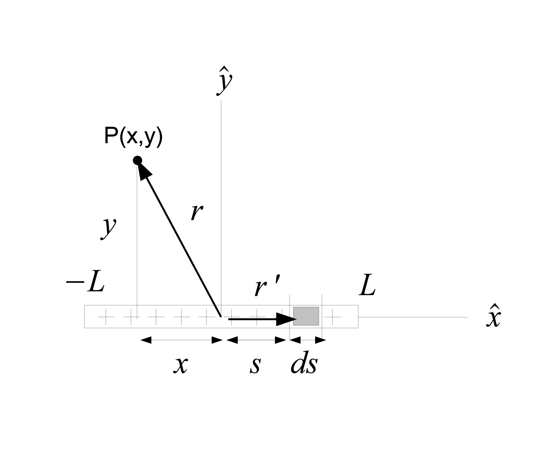
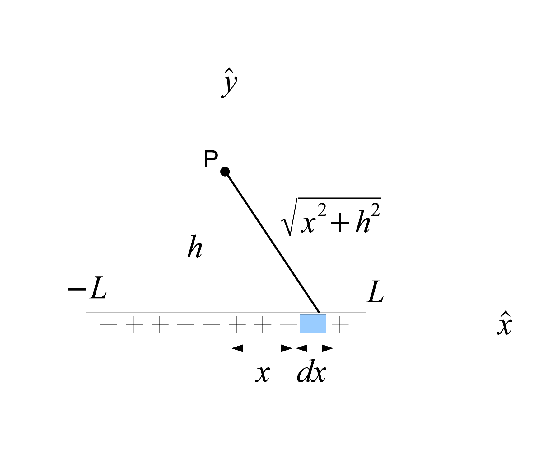
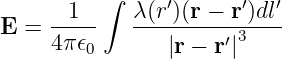
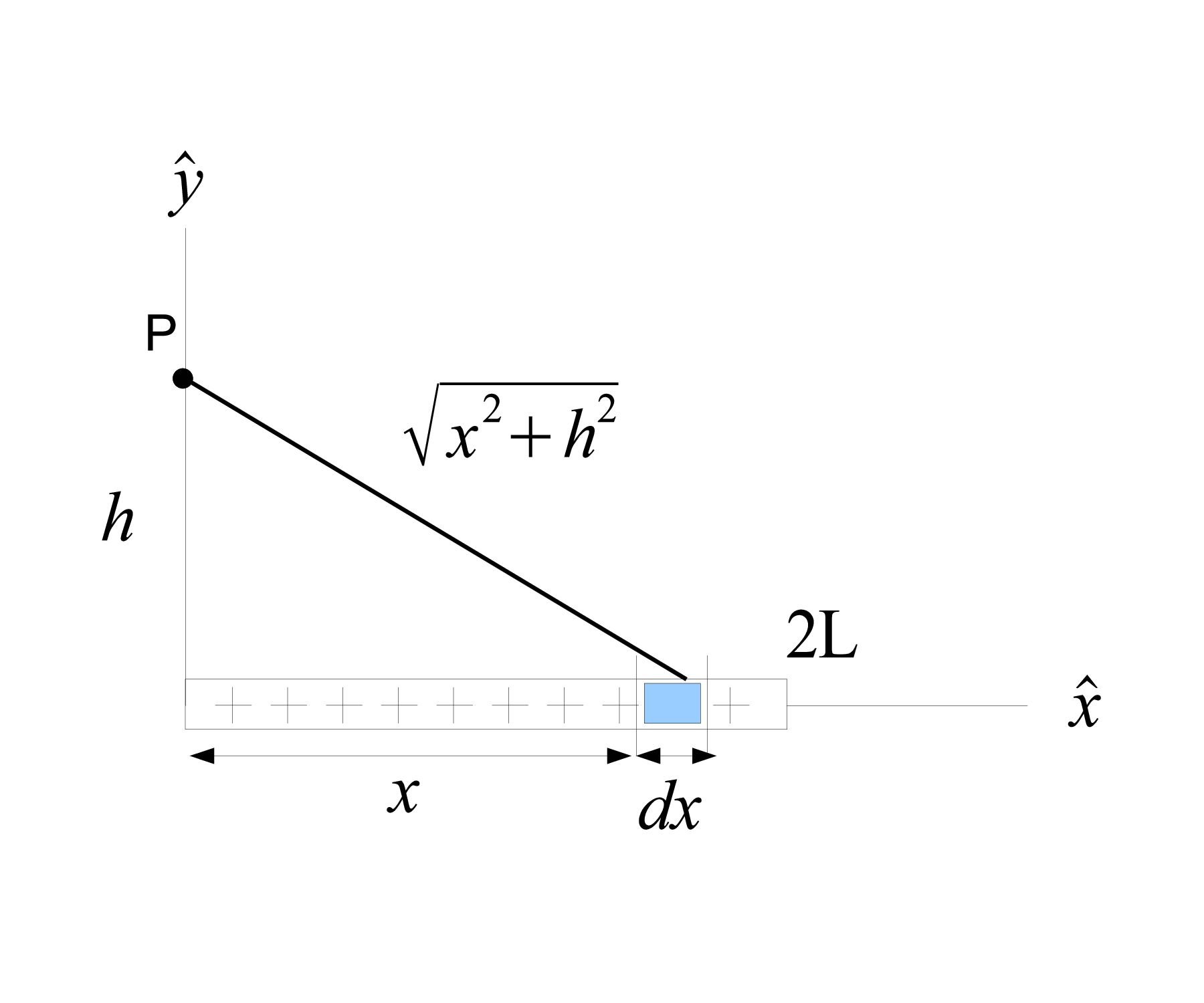
The first assumption is that the line of charge has a uniform charge density. This means that for a infinitesimal part dl’, the charge per unit length is just λ. Then, with the coordinate system setup in the figure

The vector setup is next and this is where practice is important. Try out different geometries and coordinate systems until your proficient. Remembering the convention that the prime vector is to the source point and the unprimed vector is to the field point, we get in Cartesian coordinates

Then for our integral in (1) we have

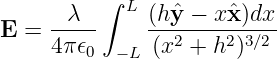
Substituting these relationships into (1)

(2)

The next step is to break the integral into its x and y components and then integrate

x component:

Usually, one looks at this setup and quickly sees the symmetry and how all the x components cancel, so it should be obvious that this integral will be zero. However, for the practice let’s go throught the motions

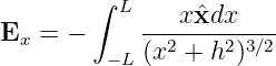Using u substitution set

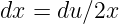notice that when we plug in the limits of integration from -L to L we get for both limits

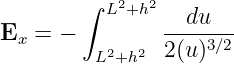however the limits of integration are the same, so we know that the integral is zero.

(3)

y component:

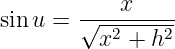
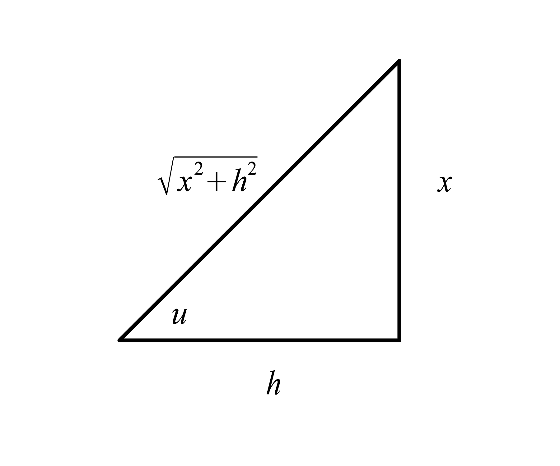
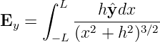This integral is a little more tricky, but is straight forward once you realize you need to use trigonometric substitution. Trig. substitution is nicely explained in [4] or any other calculus textbook. Use the right triangle in below figure to setup the needed relationships:

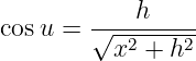
Putting all these together into the integral leaves us with

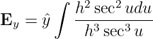simplfying

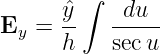but this is just

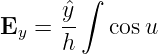Note that we can pull out the unit vector ŷ because they are constant in cartesian coordinates. Make sure that you do not do this for other coordinate systems where the unit vectors may not be constant. Carrying out this simple integration yeilds

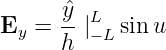we cannot simply plug in the limits of integration here, first convert back using the right triangle in figure

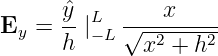Finally, evaluating this gives the the y component of the electric field.

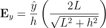Now that we know the x component is zero, the overall electric field along the center line is just in the y direction and is given by

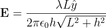
1.2 End Line

The electric field at a height h above the line segment and along the end line as shown in below figure is simliar to the previous example, except our x components of the electric field will not cancel out this time.

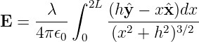
The vector setup is the same as for the center line and the only difference is the limits of integration

(4)

Once again, break the integral into its x and y components and integrate

x component:

This time the x component is non zero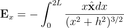

Using u substitution set

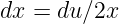notice that when we plug in the limits of integration we now get

and

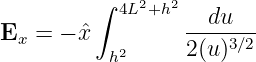integrating yields

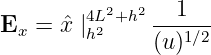finally, evaluate the limits of integration and add in the constants to get

(5)

y component:

The y component also just differs in the limits of integration so starting from previous setup

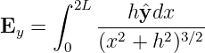which we now know gives

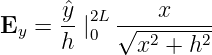Finally, evaluating this gives the the y component of the electric field.

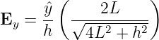Now combining x and y components with the other constants of integration, gives the overall electric field along the end line

(6)

1.3 General Solution

For the general solution of the electric field due to a line of charge, we will show off the power of the principle of superposition. Since, we know electric fields follow the principle of superposition, we can build upon simpler solutions to get a total electric field through their sums

(7)

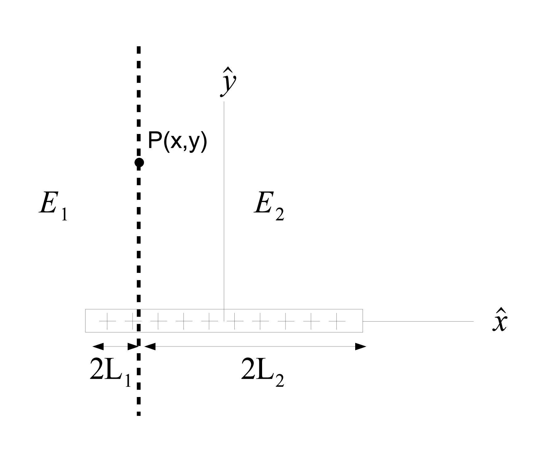
So we can now find the electric field at any point, P(x,y), in the plane by adding two cases of the earlier end line example. One electric field to handle the line of charge left of the point and one to handle the line of charge right of the point and then sum their solutions.

The key here is to get the signs correct when adding the fields and make sure we do not mix up the new terms we introduce. The relationship between the above figure and our previous analysis is

rearranging gives

(8)

(9)

Starting with the x component of equation (6) we get the electric field at P(x,y) from the left side of the line segment by inserting L = L₁ and h = y

For the right side the electric field is in the x direction is opposite to the left side and we must apply a negative sign

The total electric field in the x direction is then

(10)

Inserting equations (8) and (9) into (10) we get

(11)

Now for the y components, this time however, both the left and right side are in the same direction so we add them straight away

Once again, inserting equations (8) and (9) and a little rearranging of the signs we get

(12)

Combining equations (11) and (12), we get the total electric field at point P(x,y) due to a line segment of length 2L with the origin of the x and y coordinate frame at the center of the segment

(13)

Finally, it would be a good exercise for the reader to apply the techniques above regarding the field and source points to find the electric field directly from equation (1). The below figure displays the setup and you should get the same answer as equation (13).

[1] Reitz, J., ”Foundations of Electromagnetic Theory” Fourth Edition. Addison-Wesley Publishing Company, Inc. 1993.

[2] Griffiths, D. ”Introduction to Electrodynamics”, Prentice-Hall, Inc., 1999.

[3] Halliday, D., Resnick, R., Walker, J.: ”fundamentals of physics”. 5th Edition, John Wiley & Sons, New York, 1997.

[4] Etgen, G. ”Calculus” John Wiley & Sons, New York, 1999.