Calculus of Variations: Direct 𝜖-Expansion Exercises
This companion to CV02 develops fluency with the definition
without beginning from the memorized first-variation formula. The purpose is to make the
scalarization step automatic: construct y𝜖, substitute it into the functional, expand in powers of 𝜖,
and read the first-order coefficient.
For a sufficiently smooth scalarization,
Thus the coefficient of 𝜖 is the first variation in the chosen direction. These exercises also show why
a vanishing linear term establishes stationarity in a direction but does not, by itself, classify the
candidate.

Figure. The scalar expansion of a functional along one variation direction. The constant
term is the original functional value, the linear coefficient is the first variation, and the
quadratic coefficient contains second-order information.
1 Exercises
Exercise 1: endpoint admissibility
Let
on [a,b], where the admissible curves satisfy fixed endpoint conditions y(a) = A and
y(b) = B.
- Show that y𝜖 satisfies the same endpoint conditions for every sufficiently small 𝜖 if
η(a) = η(b) = 0.
- Show conversely that if y𝜖(a) = A and y𝜖(b) = B for all 𝜖 in an interval containing
zero, then necessarily η(a) = η(b) = 0.
Exercise 2: stationary straight line by direct expansion
Consider
with fixed endpoints y(0) = 0, y(1) = 1. Let
Construct Φ(𝜖) = J[y + 𝜖η] exactly. Find Φ(0), Φ′(0), and Φ′′(0). Interpret the result.
Exercise 3: detecting a nonstationary curve
Use the same functional and endpoint conditions as Exercise 2, but now take
Compute Φ(𝜖) exactly and determine δJ[y; η]. Explain why one nonzero first variation is sufficient
to rule out stationarity.
Exercise 4: a functional depending only on y
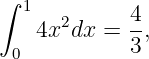
Let
and choose
Compute the exact polynomial Φ(𝜖) = J[y + 𝜖η] and find the first variation.
Exercise 5: first-order stationarity with positive quadratic change
For
use the candidate y = 0 and the fixed-endpoint variation
Find Φ(𝜖) exactly. What do the first and second derivatives at zero say?
Exercise 6: nonlinear slope functional
Let
with y(x) = x and η(x) = x(1 − x). Expand J[y + 𝜖η] through all powers of 𝜖 and compute
δJ[y; η].
Exercise 7: a total-derivative functional
Let
on the fixed-endpoint class y(0) = 0, y(1) = 1. For an arbitrary admissible variation η, directly
expand
and prove that the entire scalarized functional is independent of 𝜖. Explain the result using the
identity yy′ =  (y2∕2).
Exercise 8: two directions and linearity
Consider
at y(x) = x, with fixed-endpoint directions
- Compute δJ[x; η1] and δJ[x; η2] directly.
- Let η = αη1 + βη2. Use a direct 𝜖-expansion to verify
2 Solutions
Solution 1: endpoint admissibility
At the left endpoint,
If y(a) = A and η(a) = 0, then y𝜖(a) = A for every 𝜖. The same argument gives y𝜖(b) = B when
η(b) = 0.
Conversely, assume y𝜖(a) = A for every 𝜖 near zero. Since the unperturbed curve is
admissible,
Hence
for nonzero 𝜖 as well as zero, so η(a) = 0. Identically, η(b) = 0.
Thus fixed endpoint constraints translate directly into homogeneous endpoint conditions on
admissible variations.
Solution 2: stationary straight line by direct expansion
The perturbed curve is
and
Therefore
Expanding,
The linear integral is zero, while
Thus
and
The zero first derivative says that the straight line is stationary in this direction. The positive
second derivative says that along this particular one-parameter family, 𝜖 = 0 is a strict local
minimum. This does not yet prove a minimum against every admissible variation, although for this
functional the straight line is in fact the global minimizer.
Solution 3: detecting a nonstationary curve
Now
so
Hence
Expanding,
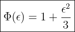
The three pieces are
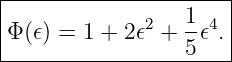
and the final integral is 1∕3. Therefore
and
Stationarity requires the first variation to vanish for every admissible direction. Finding
even one admissible η with a nonzero first variation therefore disproves stationarity
immediately.
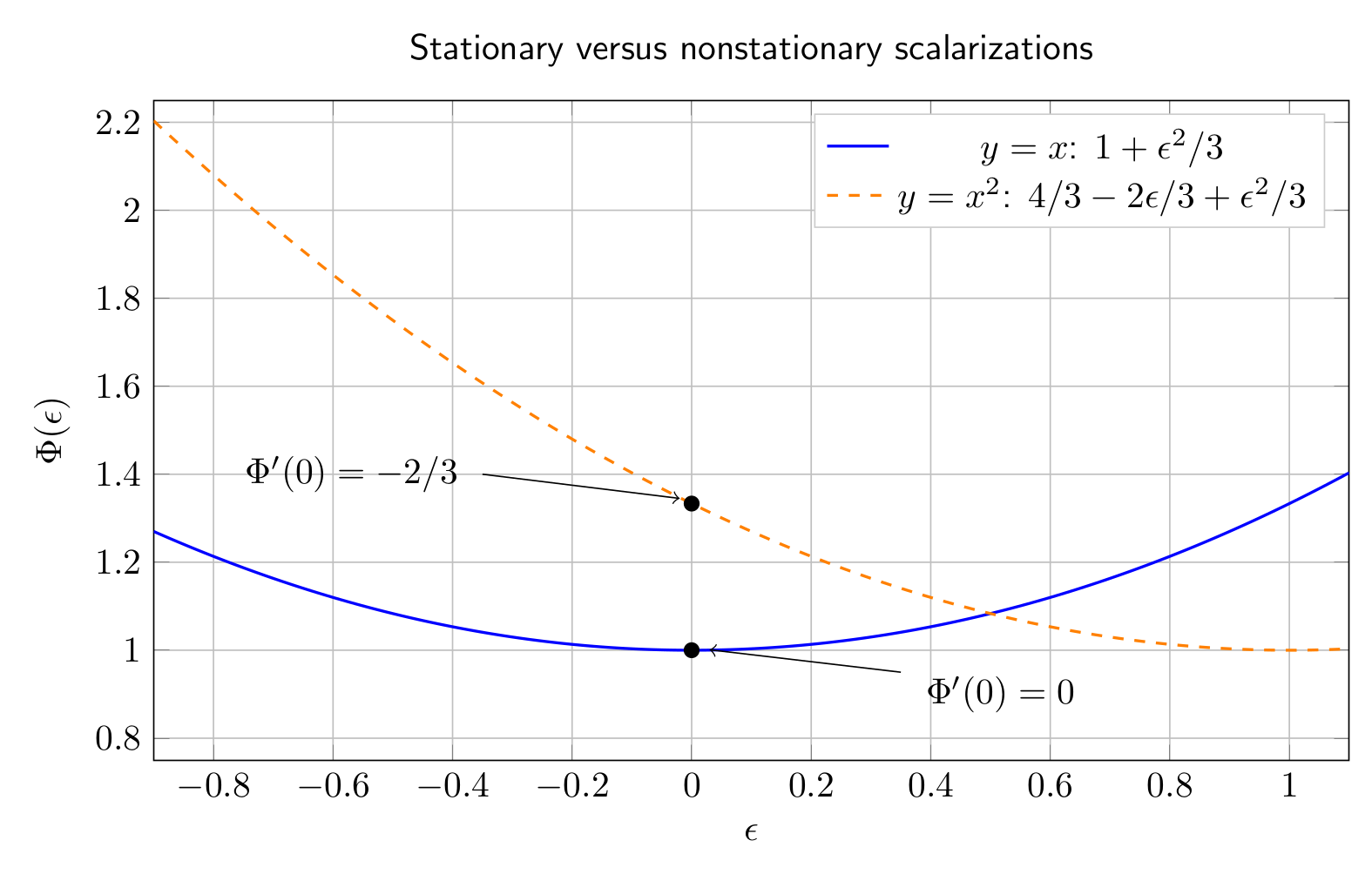
Figure. Two scalarized functionals. The straight-line candidate has a horizontal tangent at
𝜖 = 0, whereas the x2 candidate has nonzero slope there. The latter is therefore not
stationary.
Solution 4: a functional depending only on y
Substitute
Then
Expand:
The integrals are
and
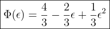
Therefore
and
Solution 5: first-order stationarity with positive quadratic change
With y = 0 and η = sin(πx),
Thus
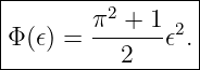
Both squared trigonometric terms integrate to 1∕2, so
Consequently,
The candidate is stationary in this direction and the cost rises quadratically for small positive or
negative 𝜖. The first derivative supplies the stationarity information; the second derivative begins
the classification question developed later in the series.
Solution 6: nonlinear slope functional
Again let
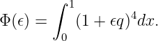
so that y𝜖′ = 1 + 𝜖q. Then
The binomial expansion gives
By symmetry about x = 1∕2,
Also,
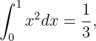
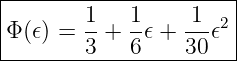
Hence
In particular,
This example shows that direct 𝜖-expansion is not restricted to quadratic functionals.
Solution 7: a total-derivative functional
Expand directly:
Therefore
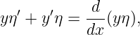
The linear integrand is a total derivative:
so fixed-endpoint variations give
Likewise,
Thus
for every admissible variation. In fact,
The value depends only on the fixed boundary data, not on the interior path.
Solution 8: two directions and linearity
For
the direct first-order expansion about y = x is
Because every admissible variation vanishes at the endpoints,
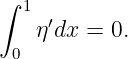
For η1 = x(1 − x),
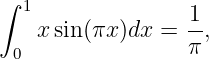
For η2 = sin(πx),
Integration by parts gives
so
Now let
The coefficient of 𝜖 in the direct expansion is
Therefore
The linearity of the first variation is therefore visible directly in the coefficient of the scalar
perturbation parameter.
3 Summary
The exercises reinforce a reliable direct procedure:
- choose an admissible perturbation η;
- form y𝜖 = y + 𝜖η;
- substitute y𝜖 and its derivatives into J;
- expand in powers of 𝜖; and
- identify the coefficient of 𝜖 as δJ[y; η].
A zero linear coefficient means stationarity in that direction. A nonzero coefficient rules out
stationarity immediately. Higher powers of 𝜖 contain classification information, but the first
variation itself is strictly a first-order object.

![[parent]](https://images.physicslibrary.org/images/uparrow.png)
![d ||
δJ [y;η ] = --J[y + 𝜖η]||
d𝜖 𝜖=0](https://images.physicslibrary.org/cache/objects/1145/make4ht/CalculusOfVariationsDirectEpsilonExpansionExercises0x.png)
![𝜖2 2
Φ (𝜖) = J[y + 𝜖η] = J [y] + 𝜖δJ [y;η] + 2 δ J[y;η] + ⋅⋅⋅ .](https://images.physicslibrary.org/cache/objects/1145/make4ht/CalculusOfVariationsDirectEpsilonExpansionExercises1x.png)

![∫
1 ′ 2
J [y] = y(x) dx
0](https://images.physicslibrary.org/cache/objects/1145/make4ht/CalculusOfVariationsDirectEpsilonExpansionExercises3x.png)


![∫ 1
J [y] = y(x)2dx,
0](https://images.physicslibrary.org/cache/objects/1145/make4ht/CalculusOfVariationsDirectEpsilonExpansionExercises6x.png)

![∫
1( ′2 2)
J[y] = y + y dx,
0](https://images.physicslibrary.org/cache/objects/1145/make4ht/CalculusOfVariationsDirectEpsilonExpansionExercises8x.png)

![∫
1 ′ 4
J[y] = y (x) dx,
0](https://images.physicslibrary.org/cache/objects/1145/make4ht/CalculusOfVariationsDirectEpsilonExpansionExercises10x.png)
![∫
1 ′
J[y] = y(x)y (x)dx
0](https://images.physicslibrary.org/cache/objects/1145/make4ht/CalculusOfVariationsDirectEpsilonExpansionExercises11x.png)
![J [y + 𝜖η]](https://images.physicslibrary.org/cache/objects/1145/make4ht/CalculusOfVariationsDirectEpsilonExpansionExercises12x.png)
![∫
1 ( 2 ′2)
J [y] = y + y dx
0](https://images.physicslibrary.org/cache/objects/1145/make4ht/CalculusOfVariationsDirectEpsilonExpansionExercises14x.png)

![δJ [x; η] = αδJ [x;η1] + βδJ [x; η2].](https://images.physicslibrary.org/cache/objects/1145/make4ht/CalculusOfVariationsDirectEpsilonExpansionExercises16x.png)





![∫
1 2
Φ (𝜖) = [1 + 𝜖(1 − 2x)] dx.
0](https://images.physicslibrary.org/cache/objects/1145/make4ht/CalculusOfVariationsDirectEpsilonExpansionExercises22x.png)





![∫
1 2
Φ (𝜖) = [2x + 𝜖(1 − 2x)] dx.
0](https://images.physicslibrary.org/cache/objects/1145/make4ht/CalculusOfVariationsDirectEpsilonExpansionExercises29x.png)


![|------------------------|
| 2 ′ 2- |
|δJ [x ;η ] = Φ (0) = − 3 .
-------------------------](https://images.physicslibrary.org/cache/objects/1145/make4ht/CalculusOfVariationsDirectEpsilonExpansionExercises34x.png)

![∫
1 2
Φ(𝜖) = [x + 𝜖x (1 − x )] dx.
0](https://images.physicslibrary.org/cache/objects/1145/make4ht/CalculusOfVariationsDirectEpsilonExpansionExercises36x.png)



![|------------|
| 1-|
δJ [x;η] = 6.|
--------------](https://images.physicslibrary.org/cache/objects/1145/make4ht/CalculusOfVariationsDirectEpsilonExpansionExercises42x.png)

![∫
2 1 [ 2 2 2 ]
Φ(𝜖) = 𝜖 π cos (πx ) + sin (πx) dx.
0](https://images.physicslibrary.org/cache/objects/1145/make4ht/CalculusOfVariationsDirectEpsilonExpansionExercises44x.png)





![|------------|
-δJ[x;η] =-0.-](https://images.physicslibrary.org/cache/objects/1145/make4ht/CalculusOfVariationsDirectEpsilonExpansionExercises53x.png)
![∫
1 ′ ′
J [y + 𝜖η] = (y + 𝜖η)(y + 𝜖η )dx.
0](https://images.physicslibrary.org/cache/objects/1145/make4ht/CalculusOfVariationsDirectEpsilonExpansionExercises54x.png)
![∫ 1 ∫ 1
J[y + 𝜖η] = J [y ] + 𝜖 (yη ′ + y′η)dx + 𝜖2 ηη′dx.
0 0](https://images.physicslibrary.org/cache/objects/1145/make4ht/CalculusOfVariationsDirectEpsilonExpansionExercises55x.png)
![∫ 1
(yη′ + y′η)dx = [yη]10 = 0.
0](https://images.physicslibrary.org/cache/objects/1145/make4ht/CalculusOfVariationsDirectEpsilonExpansionExercises57x.png)
![∫
1 ′ 1- 21
ηη dx = 2[η ]0 = 0.
0](https://images.physicslibrary.org/cache/objects/1145/make4ht/CalculusOfVariationsDirectEpsilonExpansionExercises58x.png)
![|----------------|
|J[y + 𝜖η] = J[y]|
-----------------](https://images.physicslibrary.org/cache/objects/1145/make4ht/CalculusOfVariationsDirectEpsilonExpansionExercises59x.png)
![∫ ( )
1 d-- 1-2 1- 2 2 1-
J[y] = dx 2y dx = 2[y(1) − y (0)] = 2 .
0](https://images.physicslibrary.org/cache/objects/1145/make4ht/CalculusOfVariationsDirectEpsilonExpansionExercises60x.png)
![∫ 1
J[y] = (y2 + y′2)dx,
0](https://images.physicslibrary.org/cache/objects/1145/make4ht/CalculusOfVariationsDirectEpsilonExpansionExercises61x.png)
![∫
1 ′ 2
J[x + 𝜖η] = J [x] + 2𝜖 (xη + η )dx + O(𝜖 ).
0](https://images.physicslibrary.org/cache/objects/1145/make4ht/CalculusOfVariationsDirectEpsilonExpansionExercises62x.png)
![∫ 1 |--|
δJ[x;η1] = 2 x2(1 − x)dx = |1-.
0 -6-|](https://images.physicslibrary.org/cache/objects/1145/make4ht/CalculusOfVariationsDirectEpsilonExpansionExercises64x.png)
![∫
1
δJ[x;η2] = 2 xsin(πx )dx.
0](https://images.physicslibrary.org/cache/objects/1145/make4ht/CalculusOfVariationsDirectEpsilonExpansionExercises65x.png)
![|-----------2--|
|δJ[x;η2] = --.|
------------π--|](https://images.physicslibrary.org/cache/objects/1145/make4ht/CalculusOfVariationsDirectEpsilonExpansionExercises67x.png)


![|------------------------------------------|
-δJ[x;α-η1 +-β-η2] =-α-δJ-[x;-η1] +-β-δJ[x;η2].](https://images.physicslibrary.org/cache/objects/1145/make4ht/CalculusOfVariationsDirectEpsilonExpansionExercises70x.png)