|
|
|
|||||||
under the boundary conditions  We first try to separate the variables, i.e. seek the solution of (1) of the form  Then we get  and thus (1) gets the form
and the boundary conditions  We separate the variables in (2): 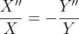 This equation is not possible unless both sides are equal to a same negative constant −k2, which implies for X′′ = −k2X the solution  and for Y ′′ = k2Y the solution  The two first boundary conditions give 0 = X(0) = C1, 0 = X(π) = 0 + C2 sin kπ, and since C2≠0, we must have sin kπ = 0, i.e.  Therefore  The fourth boundary condition now gives that 0 = Y ′(0) = nD2; thus D2 = 0 and Y (y) := D1 cosh ny. So (1) has infinitely many solutions
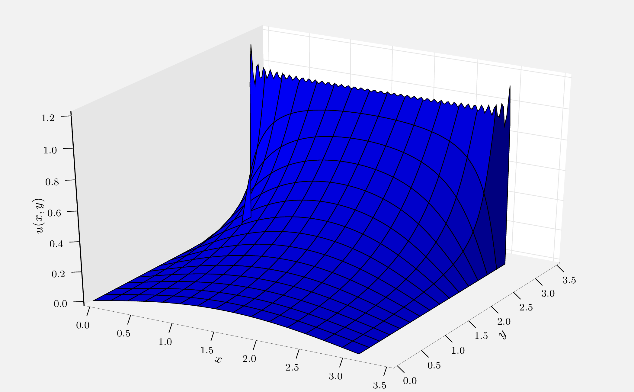
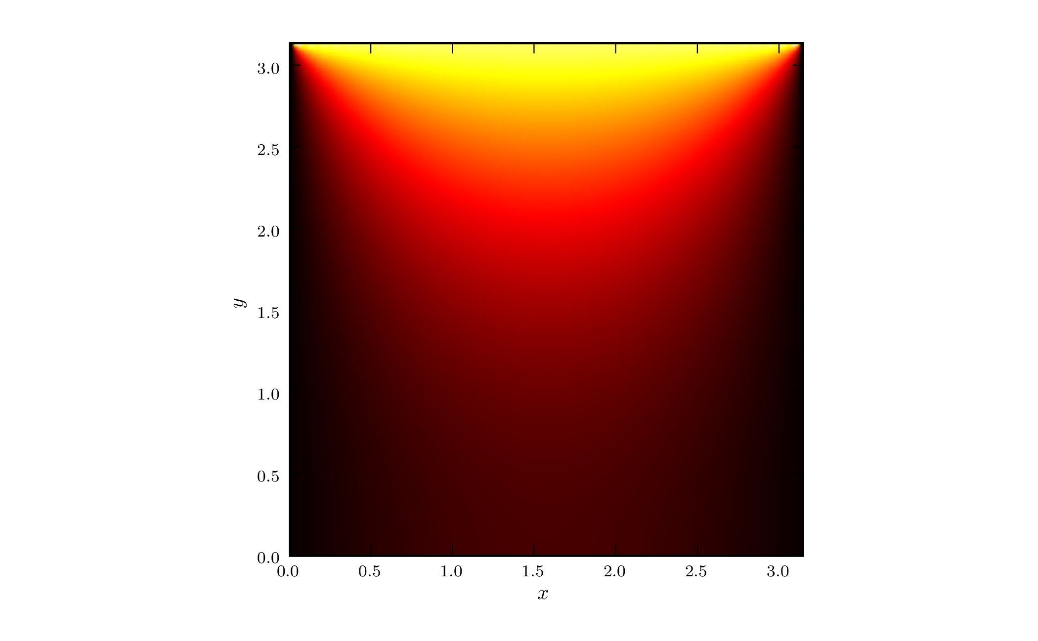
with n ∈ ℤ+ and they all satisfy the boundary conditions except the third. Because of the linearity of (1), also the sum 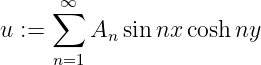 of the functions (3) satisfy (1) and those boundary conditions, provided that this series converges. The third boundary condition requires that  on the interval 0 ≦ x ≦ π. But this is the Fourier sine series of the constant function x  The even n’s here give 0 and the odd give  Thus we obtain the solution  It can be shown that this series converges in the whole square of the plate. Visualization of the solution
Remark. The function u has been approximated in the plot by computing a partial sum of the true infinite-series solution. However, there is substantial numerical error in the approximate solution near y = π, evident in the small oscillations observed in the surface plot, that should not be there in theory. This phenomenon is actually inevitable given that the boundary conditions are actually discontinuous at the corners (0, π) and (π, π). More precisely, observe that when y = π, the formula for u(x, y) reduces to the Fourier series  for the discontinuous function on [−π, π]:
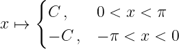 That means the Fourier expansion will necessarily be subject to the Gibbs phenomenon. Of course, the series also cannot converge absolutely; in other words, the terms of the series decay too slowly in magnitude, adversely affecting the numerical solution. "example of solving the heat equation" is owned by bloftin. This object's parent. Cross-references: magnitude, Fourier series, small oscillations, partial sum, boundary, function, temperature There is 1 reference to this object. This is version 1 of example of solving the heat equation, born on 2007-08-11. Object id is 260, canonical name is ExampleOfSolvingTheHeatEquation. Accessed 2936 times total. Classification:
|
|
|
|
Pending Errata and AddendaNone.
|
DiscussionNo messages.
|
Interact |
![[parent]](https://images.physicslibrary.org/images/uparrow.png)