
|
|
|
|||||||
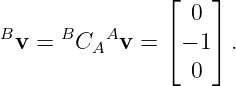
Thus
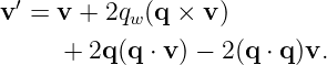
 Equation (21) gives
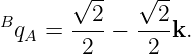
Apply it to the fixed vector with A coordinates
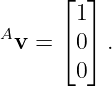 Then
This agrees with the quaternion sandwich developed in the preceding PhysicsLibrary article.
8 What the columns meanBecause
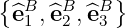
 the columns of BC A have an immediate geometric interpretation. Let the standard basis columns in frame A be
 Applying the passive coordinate transformation gives
Thus:
For example,
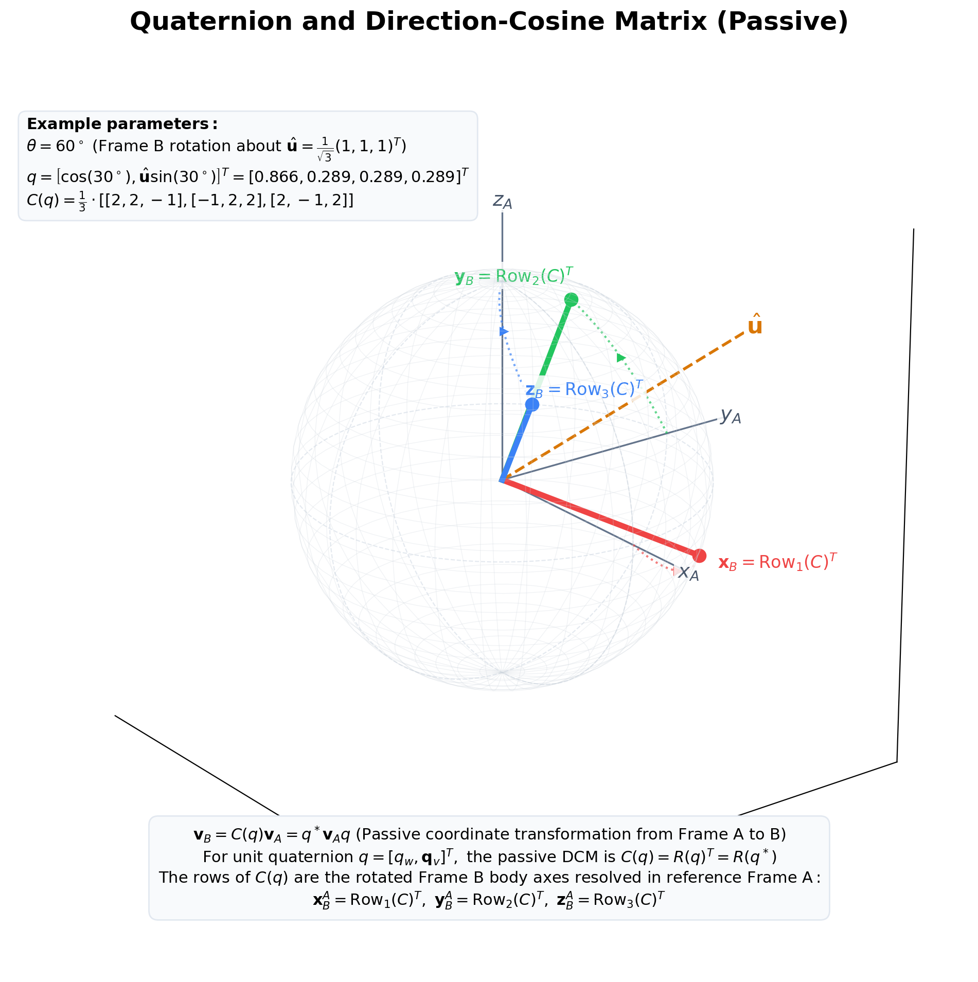
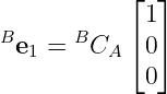 is simply the first column of BC A. The following illustration shows this column interpretation for a representative unit quaternion and its passive direction cosine matrix.
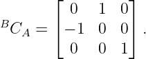
Figure. A unit quaternion and its passive direction cosine matrix. The original A frame basis directions are shown together with their coordinate representations in frame B. The three columns of BC A are Be 1, Be 2, and Be 3. This interpretation is also a useful convention check. For the positive 90∘ passive frame rotation about +z,
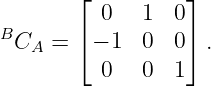 Its first column is
 which agrees with the passive coordinate result

9 Conjugate and transposeThe quaternion conjugate reverses the frame map:
 The corresponding matrix relation is
Therefore
Since a proper DCM is orthogonal,
Thus quaternion conjugation, quaternion inversion, matrix transposition, and matrix inversion all describe the same reversal of a unit frame transformation.
10 Quaternion and DCM compositionSuppose
 maps A coordinates into B coordinates, and
 maps B coordinates into C coordinates. The quaternion chain is
 Apply the quaternion to matrix map:
 Equation (19) is chosen so that Hamilton multiplication is homomorphic:
Therefore
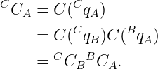 Hence
The quaternion and DCM frame chains have identical written order.
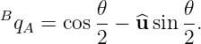
11 Why some sources show the transpose formulaA different source may use the same Hamilton quaternion coefficients but assign the quaternion to the opposite frame map or to an active vector rotation. For the same positive geometric rotation, the active rotor is
 Its active rotation matrix is
Therefore two sources may display matrix formulas that are transposes of one another while describing the same physical orientation from inverse viewpoints. A quaternion to DCM formula should never be copied without its frame direction and sandwich convention.
12 The
|
 | (32) |
The map from unit quaternions to proper rotation matrices is two to one.
This is not a numerical defect. It is an intrinsic property of the quaternion representation of three dimensional orientation.
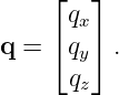
Let
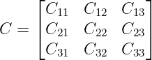
be a proper DCM that obeys the PhysicsLibrary passive mapping convention.
From equation (20),

Therefore
 | (33) |
When qw is safely away from zero, select one quaternion sign and compute
 | (34) |
The off diagonal differences give
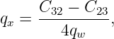 | (35) |
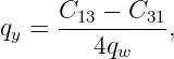 | (36) |
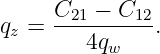 | (37) |
These signs are consistent with the PhysicsLibrary passive DCM formula in equation (20).
For a frame rotation near 180∘,
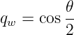
is near zero.
The formulas in equations (36) through (38) then divide by a small number. The mathematics remains valid, but the numerical calculation becomes poorly conditioned.
A robust implementation instead chooses the quaternion component associated with the largest diagonal expression.
Let

If t > 0, define
 | (38) |
Then
 | (39) |
 | (40) |
If C11 is the largest diagonal term, define
 | (41) |
Then
 | (42) |
 | (43) |
If C22 is the largest diagonal term, define
 | (44) |
Then
 | (45) |
 | (46) |
Otherwise use the qz branch:
 | (47) |
Then
 | (48) |
 | (49) |
Each branch returns one member of the equivalent pair q and −q.
After extraction, numerical software should normally normalize the quaternion to remove roundoff error.
Consider a positive frame rotation of 60∘ about
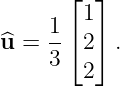
The passive quaternion is
 | (50) |
Substitution into equation (20) gives
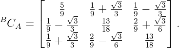 | (51) |
The trace is
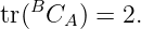
Therefore equation (35) gives
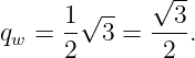
The vector components recover as

Thus the DCM to quaternion conversion returns the original passive quaternion.
Choosing the opposite overall quaternion sign would produce the same DCM.
For a quaternion generated matrix,

For unit q,

Using the homomorphism property,
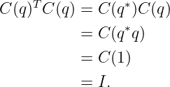
Therefore
 | (52) |
This gives a compact quaternion proof of DCM orthogonality.
An orthogonal matrix has determinant +1 or −1.
At the identity quaternion,

we have

and therefore

Unit quaternions vary continuously, and the determinant of an orthogonal matrix cannot change continuously from +1 to −1 without passing through zero. An orthogonal matrix never has zero determinant.
Therefore every unit quaternion generates a proper rotation matrix:
 | (53) |
A numerical matrix intended to represent orientation should satisfy
 | (54) |
and
 | (55) |
Measured or numerically propagated matrices may drift slightly away from these conditions.
Converting a badly nonorthogonal matrix directly to a quaternion can produce misleading results. If the deviation is more than roundoff level, the matrix should first be examined or projected back onto SO(3) using a suitable orthogonalization method.
The quaternion extraction formulas assume that the input is already a proper rotation matrix.
For software validation, perform both conversion directions.
Starting with a normalized quaternion q:

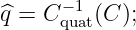
Because q and −q represent the same orientation, a useful scalar check is
 | (56) |
Alternatively compare

with

Starting with a DCM C, perform the reverse round trip

and verify that the matrices agree to numerical tolerance.
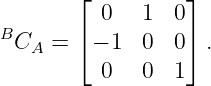
The positive 90∘ frame rotation about +z provides a compact convention test.
PhysicsLibrary expects
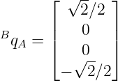 | (57) |
and
 | (58) |
Therefore
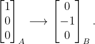 | (59) |
If a library instead produces
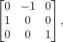
it is producing the inverse matrix for this declared passive frame transformation, or equivalently the positive active rotation matrix.
This one case detects many transpose and sign mistakes immediately.
Two valid formulas may be transposes of one another because they represent inverse maps.
For the same positive physical geometry, the active rotor is the conjugate of the canonical passive frame quaternion.
PhysicsLibrary keeps Hamilton multiplication and uses the quaternion to DCM assignment in equation (19), for which

 and
and  should produce different matrices.
They must produce exactly the same DCM.
 .
.
When qw is small, use the largest component branch instead.
Small floating point errors can move the result slightly away from unit norm.
 .
.
The conversion formulas assume an orthogonal matrix with determinant +1.
A recovered quaternion may equal −q and still represent the identical orientation.
Array layout does not determine frame direction, active or passive meaning, or the multiplication law.
The preceding article, composition of rotations and quaternion order, establishes the passive frame chain

The present article derives the matrix representation whose frame chain uses the same written order.
A separate companion entry, Quaternions and Direction Cosine Matrices: Examples, Exercises, and Solutions, provides the Q09E self study problem bank.
The next main article, quaternions and Euler angles, uses the quaternion and DCM formulas developed here to derive the intrinsic 3-2-1 yaw, pitch, roll conversion under the same passive convention.
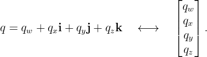
The quaternion to matrix relation follows directly from the Hamilton sandwich product. The principal engineering difficulty is convention management: different sources may use inverse frame maps, active vector rotations, transposed DCMs, scalar last storage, or flipped quaternion multiplication.
Sommer and coauthors provide a modern discussion of the Hamilton and flipped multiplication conventions and explain how quaternion to matrix assignments interact with passive frame mappings. Moore provides an openly licensed engineering treatment of reference frames and direction cosine matrices. Henderson’s Shuttle era memorandum is a useful historical engineering reference for explicit relationships among Euler Angles, quaternions, and transformation matrices.
[1] H. Sommer, I. Gilitschenski, M. Bloesch, S. Weiss, R. Siegwart, and J. Nieto, “Why and How to Avoid the Flipped Quaternion Multiplication,” Aerospace, vol. 5, no. 3, article 72, 2018. Published under CC BY 4.0. Publisher article
[2] J. K. Moore, Learn Multibody Dynamics, chapter “Orientation of Reference Frames.” Distributed under CC BY 4.0. Learn Multibody Dynamics
[3] D. M. Henderson, Euler Angles, Quaternions, and Transformation Matrices: Working Relationships, JSC-12960, NASA Johnson Space Center, Mission Planning and Analysis Division, 1977. Engineering reference. NASA Technical Reports Server search
[4] W. R. Hamilton, Elements of Quaternions, 2nd ed., edited by C. J. Joly, Longmans, Green, and Co., 1899. Public domain historical source. Internet Archive scan
Unless otherwise noted, this PhysicsLibrary entry is intended for release under the Creative Commons Attribution ShareAlike 4.0 International license.
| Keywords: | quaternion, direction cosine matrix, DCM, rotation matrix, active rotation, passive rotation, frame transformation, attitude matrix |
|
| Physics Classification: | 02.40.Yy (Geometric mechanics ) |
| 02.10.Hh (Rings and algebras) | |
| 45.40.-f (Dynamics and kinematics of rigid bodies) |
None.
No messages.











![[BC ] = ^eB ⋅^eA .
A ij i j](https://images.physicslibrary.org/cache/objects/1101/make4ht/QuaternionsAndDirectionCosineMatrices14x.png)









![⌊ ⌋
0 − qz qy
[q ]× = ⌈ qz 0 − qx⌉ ,
− qy qx 0](https://images.physicslibrary.org/cache/objects/1101/make4ht/QuaternionsAndDirectionCosineMatrices26x.png)
![[q]×v = q × v.](https://images.physicslibrary.org/cache/objects/1101/make4ht/QuaternionsAndDirectionCosineMatrices27x.png)

![[( ) ]
v′ = q2− qTq I + 2qqT + 2qw[q]× v.
w](https://images.physicslibrary.org/cache/objects/1101/make4ht/QuaternionsAndDirectionCosineMatrices29x.png)
![C (q) = (q2 − qT q)I + 2qqT + 2q [q] .
w w ×](https://images.physicslibrary.org/cache/objects/1101/make4ht/QuaternionsAndDirectionCosineMatrices30x.png)




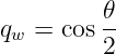
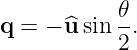


![2qw[q]× = − sin 𝜃[^u ]×,](https://images.physicslibrary.org/cache/objects/1101/make4ht/QuaternionsAndDirectionCosineMatrices39x.png)
![BCA = I cos 𝜃 + (1 − cos 𝜃)^u^uT − [^u ]× sin 𝜃.](https://images.physicslibrary.org/cache/objects/1101/make4ht/QuaternionsAndDirectionCosineMatrices40x.png)
 frame rotation about

![[ ]
BCA = Be1 Be2 Be3 .](https://images.physicslibrary.org/cache/objects/1101/make4ht/QuaternionsAndDirectionCosineMatrices51x.png)






 versus
  ambiguity